sigmoid <- function(z) 1 / (1 + exp(-z))

neuron <- function(stress, support) {
  sigmoid(-4 + 1.2 * stress - 0.8 * support)
}

neuron(stress = 4, support = 2)
[1] 0.3100255neuron(stress = 2, support = 4)[1] 0.008162571Neural networks are the method behind most of what is called artificial intelligence today: image recognition, speech recognition, translation, and the large language models of Chapter 18. Their reputation leads many researchers to assume that a neural network must predict better than a traditional model on any data. The assumption deserves to be tested rather than accepted, and testing it requires understanding what a neural network is. The answer is less mysterious than the reputation suggests: a neural network is built from units that each perform a logistic regression, and it learns by repeatedly adjusting its weights to reduce its errors.
This chapter builds a neural network from a single “neuron”, shows by hand what training does, fits a network to the dropout data with the same tidymodels workflow as Chapters 11 and 12, and compares it fairly with the simpler models. It ends with deep learning: what it is, when it helps, and where to learn more. In the story, a member of Elaf’s research group asks why she does not simply use AI, since a neural network would surely do better than logistic regression, and her supervisor suggests that she find out, carefully.
mlp()), using weight decay to prevent overfitting.A neuron (or unit) in a neural network does three things. It multiplies each input by a weight, adds up the results together with a constant called the bias, and passes the total through an activation function, which turns it into the neuron’s output.
Take a neuron with two inputs, a student’s stress and support scores, with weights 1.2 and −0.8 and a bias of −4. For a student with stress 4 and support 2, the total is
\[ -4 + 1.2 \times 4 - 0.8 \times 2 = -0.8. \]
The activation function here is the sigmoid (also called the logistic function), which squeezes any number into the range 0 to 1:
\[ \text{sigmoid}(z) = \frac{1}{1 + e^{-z}}. \]
In R:
sigmoid <- function(z) 1 / (1 + exp(-z))
neuron <- function(stress, support) {
sigmoid(-4 + 1.2 * stress - 0.8 * support)
}
neuron(stress = 4, support = 2)[1] 0.3100255neuron(stress = 2, support = 4)[1] 0.008162571The high-stress, low-support student gets an output of 0.31; the low-stress, high-support student, 0.008. If the output is read as the probability of considering dropout, this neuron is exactly a logistic regression (Chapter 8): the bias is the intercept, the weights are the coefficients, and the sigmoid turns the log odds into a probability. Everything a single neuron can do, Chapter 8 has already done.
The power of neural networks comes from connecting many neurons in layers. In the most common design, the multilayer perceptron, the inputs feed into a hidden layer of neurons, each with its own weights; the outputs of the hidden neurons then feed into an output layer, which produces the prediction. Figure 15.1 shows a network with three inputs and three hidden neurons.
flowchart LR
  I1((Stress)) --> H1((H1))
  I1 --> H2((H2))
  I1 --> H3((H3))
  I2((Support)) --> H1
  I2 --> H2
  I2 --> H3
  I3((Sleep)) --> H1
  I3 --> H2
  I3 --> H3
  H1 --> O((P of<br/>dropout))
  H2 --> O
  H3 --> O
Each hidden neuron learns its own combination of the inputs: one might respond to high stress, another to the combination of low support and short sleep. The output neuron then combines these. Because each neuron applies a curved activation function, the network as a whole can represent curved relationships and interactions that a single logistic regression cannot. With enough hidden neurons, a network can approximate almost any relationship between inputs and output. That flexibility is its strength, and, as you will see, its danger.
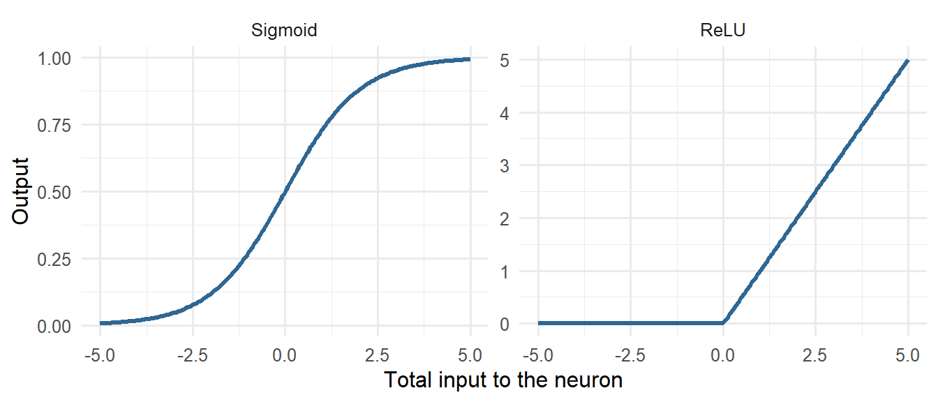
The activation function matters. Figure 15.2 shows the two most common: the sigmoid, used in this chapter, and the ReLU (rectified linear unit), which simply replaces negative totals with zero and is the standard choice in deep networks.
A network starts with small random weights, so its first predictions are useless. Training adjusts the weights step by step to reduce the prediction error on the training data. At each step, an algorithm works out, for every weight, whether a small increase or decrease would reduce the error (the gradient), and moves all the weights a little in the helpful direction. This is gradient descent. One pass through the training data is an epoch, and training usually runs for hundreds of epochs.
The idea is clearest when one step is worked by hand. Take a single neuron, which is a logistic regression, and six students, with their stress measured from the group’s average:
six <- data.frame(stress  = c(2.0, 2.5, 3.0, 3.5, 4.0, 4.5) - 3.25,
                  dropout = c(0,   0,   1,   0,   1,   1))
The error to be reduced is the log loss, the measure of fit that logistic regression uses: it is small when the neuron gives high probabilities to the students who did consider dropping out and low probabilities to those who did not. Training starts with both weights at zero, so every student receives a probability of 0.5:
log_loss <- function(b0, b1) {
  p <- sigmoid(b0 + b1 * six$stress)
  -mean(six$dropout * log(p) + (1 - six$dropout) * log(1 - p))
}

b0 <- 0
b1 <- 0
log_loss(b0, b1)
[1] 0.6931472For this neuron, the gradient has a simple form: for each weight, the average of the prediction errors (predicted probability minus the actual outcome), each multiplied by the input that the weight belongs to (1 for the bias):
p <- sigmoid(b0 + b1 * six$stress)
gradient_b0 <- mean(p - six$dropout)
gradient_b1 <- mean((p - six$dropout) * six$stress)
c(gradient_b0, gradient_b1)
[1] 0.0000000 -0.2916667The gradient for the stress weight is negative, which means that increasing the weight would reduce the error: the students who considered dropping out have higher stress, and the neuron does not yet know it. One step of gradient descent moves each weight against its gradient, by an amount set by the learning rate:
learning_rate <- 1
b0 <- b0 - learning_rate * gradient_b0
b1 <- b1 - learning_rate * gradient_b1
c(b0 = b0, b1 = b1, loss = log_loss(b0, b1))
b0 b1 loss
0.0000000 0.2916667 0.6157970 After one step, the stress weight has become positive and the loss has fallen from 0.693 to 0.616. Training is nothing more than this step, repeated. The loop below repeats it 2,000 times and records the loss:
b0 <- 0
b1 <- 0
loss_history <- numeric(2000)
for (step in 1:2000) {
  p  <- sigmoid(b0 + b1 * six$stress)
  b0 <- b0 - learning_rate * mean(p - six$dropout)
  b1 <- b1 - learning_rate * mean((p - six$dropout) * six$stress)
  loss_history[step] <- log_loss(b0, b1)
}
rbind(gradient_descent = c(b0, b1),
      glm = coef(glm(dropout ~ stress, data = six, family = binomial)))
(Intercept) stress
gradient_descent 6.111907e-17 2.428055
glm -1.790641e-16 2.428055ggplot(data.frame(step = 1:2000, loss = loss_history), aes(x = step, y = loss)) +
geom_line(colour = "#2f6793", linewidth = 1) +
scale_x_log10() +
labs(x = "Training step", y = "Log loss") +
theme_minimal(base_size = 12)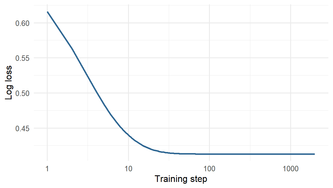
After 2,000 small steps, the weights found by gradient descent are the coefficients that R’s glm() calculates for the same logistic regression. A neural network with thousands of weights is trained in exactly this way. The gradients are harder to write down, and a method called backpropagation calculates them efficiently, but each step still moves every weight a little in the direction that reduces the error.
Two consequences follow. First, because training starts from random weights, two runs can give slightly different networks, so set.seed() matters. Second, a network with many weights can keep reducing its training error long after it has learned the real pattern, by memorising the noise. The usual defence is weight decay: a penalty on large weights, exactly like the ridge penalty of Chapter 13. In tidymodels it is called penalty.
The data, split, recipe, and folds are those of Chapters 11 and 12. Neural networks need normalised inputs, like the penalised regressions of Chapter 13, and the recipe already provides them.
library(tidymodels)
tidymodels_prefer()

scores <- questionnaire |>
  mutate(
    stress_4     = 6 - stress_4,
    stress       = rowMeans(pick(stress_1:stress_6), na.rm = TRUE),
    burnout      = rowMeans(pick(burnout_1:burnout_6), na.rm = TRUE),
    support      = rowMeans(pick(support_1:support_6), na.rm = TRUE),
    satisfaction = rowMeans(pick(satisfaction_1:satisfaction_4), na.rm = TRUE)
  ) |>
  select(student_id, stress, burnout, support, satisfaction)

dropout_data <- students |>
  left_join(scores, join_by(student_id)) |>
  left_join(semesters |> filter(semester == 1) |> select(-semester), join_by(student_id)) |>
  mutate(considering_dropout = factor(considering_dropout, levels = c("Yes", "No"))) |>
  select(-student_id, -supervisor_id, -workshop, -workshop_sessions)

set.seed(2026)
dropout_split <- initial_split(dropout_data, prop = 0.75, strata = considering_dropout)
dropout_train <- training(dropout_split)
dropout_test  <- testing(dropout_split)

dropout_recipe <- recipe(considering_dropout ~ ., data = dropout_train) |>
  step_impute_median(all_numeric_predictors()) |>
  step_dummy(all_nominal_predictors()) |>
  step_normalize(all_numeric_predictors())

set.seed(2026)
dropout_folds <- vfold_cv(dropout_train, v = 10, strata = considering_dropout)
In tidymodels, a multilayer perceptron is mlp(). Its main arguments are hidden_units (the number of neurons in the hidden layer), penalty (the weight decay), and epochs. The nnet engine, which comes with R, fits networks with one hidden layer; MaxNWts raises its limit on the number of weights.
A network with 20 hidden neurons and no weight decay comes first, as a warning:
big_net <- mlp(hidden_units = 20, penalty = 0, epochs = 1000) |>
  set_engine("nnet", MaxNWts = 5000) |>
  set_mode("classification")

set.seed(2026)
big_fit <- fit(workflow(dropout_recipe, big_net), data = dropout_train)

augment(big_fit, new_data = dropout_train) |> roc_auc(considering_dropout, .pred_Yes)
# A tibble: 1 × 3
.metric .estimator .estimate
<chr> <chr> <dbl>
1 roc_auc binary 1augment(big_fit, new_data = dropout_test) |> roc_auc(considering_dropout, .pred_Yes)# A tibble: 1 × 3
.metric .estimator .estimate
<chr> <chr> <dbl>
1 roc_auc binary 0.641A perfect AUC on the training data, and 0.64 on new students: the same overfitting as the one-nearest-neighbour model of Chapter 11. The network has 521 weights and only 449 training students, so it has more than enough freedom to memorise every one of them.
The number of hidden neurons and the weight decay are hyperparameters, tuned with cross-validation as in Chapters 11 to 13. Weight decay is tried on a logarithmic scale from 0.01 to about 30:
net_spec <- mlp(hidden_units = tune(), penalty = tune(), epochs = 500) |>
  set_engine("nnet", MaxNWts = 5000) |>
  set_mode("classification")

net_wf <- workflow(dropout_recipe, net_spec)

net_grid <- expand_grid(hidden_units = c(1, 3, 5, 10, 20),
                        penalty = 10^seq(-2, 1.5, by = 0.5))

set.seed(2026)
net_tuning <- tune_grid(net_wf, resamples = dropout_folds, grid = net_grid,
metrics = metric_set(roc_auc))autoplot(net_tuning) + theme_minimal(base_size = 12)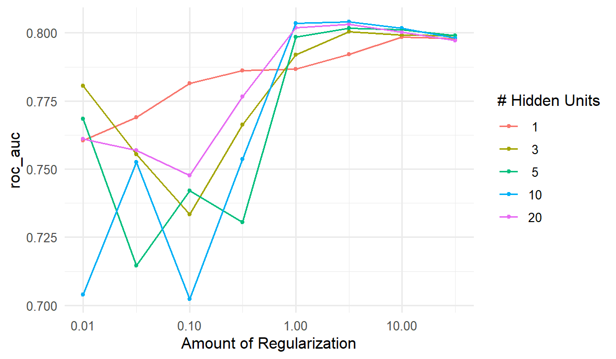
Figure 15.4 tells a clear story. With little weight decay, the networks overfit, and the bigger networks overfit most. With enough weight decay, networks of every size do about equally well. The penalty, not the size, is what matters most here.
show_best(net_tuning, metric = "roc_auc", n = 3)# A tibble: 3 × 8
hidden_units penalty .metric .estimator mean n std_err .config
<dbl> <dbl> <chr> <chr> <dbl> <int> <dbl> <chr>
1 10 3.16 roc_auc binary 0.804 10 0.0300 pre0_mod30_post0
2 10 1 roc_auc binary 0.804 10 0.0298 pre0_mod29_post0
3 20 3.16 roc_auc binary 0.803 10 0.0299 pre0_mod38_post0best_net <- select_best(net_tuning, metric = "roc_auc")The best network has a cross-validated AUC of 0.804. For comparison, logistic regression on the same folds:
set.seed(2026)
logistic_cv <- fit_resamples(workflow(dropout_recipe, logistic_reg()),
                             resamples = dropout_folds, metrics = metric_set(roc_auc))
collect_metrics(logistic_cv)
# A tibble: 1 × 6
.metric .estimator mean n std_err .config
<chr> <chr> <dbl> <int> <dbl> <chr>
1 roc_auc binary 0.804 10 0.0303 pre0_mod0_post0The two are practically identical: 0.804 for the network and 0.804 for logistic regression. The final test on the held-out students confirms it:
set.seed(2026)
final_net <- net_wf |>
  finalize_workflow(best_net) |>
  last_fit(dropout_split, metrics = metric_set(roc_auc, accuracy))
collect_metrics(final_net)
# A tibble: 2 × 4
.metric .estimator .estimate .config
<chr> <chr> <dbl> <chr>
1 accuracy binary 0.841 pre0_mod0_post0
2 roc_auc binary 0.853 pre0_mod0_post0The network reaches a test AUC of 0.85, against 0.84 for logistic regression on the same test students (Chapter 11). With only 151 test students, of whom 23 considered dropping out, a difference of this size is well within chance. The answer to the research group is therefore that a neural network does not predict dropout better. Chapters 12 and 13 found the same for random forests, support vector machines, and boosting. The wellbeing data has a smooth pattern, which logistic regression captures fully, leaving nothing extra for a more flexible model to find.
And the neural network has real costs. Even the tuned network, with 10 hidden neurons, has 261 weights, which cannot be interpreted: there is no equivalent of an odds ratio saying how much each predictor matters. Without strong weight decay, its results depend on the random starting weights. And it needed careful tuning to avoid overfitting. Logistic regression is kept, and the thesis reports that a neural network was tried and did not improve on it, which is itself a useful finding.
Neural networks are not magic, but they are not overrated either; they are powerful in particular situations. They excel with unstructured data, such as images, sound, and text, where the raw inputs (pixels, sound samples, words) mean little on their own and the useful features must be learned from them; here they outperform every other method by a wide margin. They need very large datasets, with many thousands or millions of cases, to fit models with thousands of weights reliably. And they can capture complex, non-linear relationships that simpler models miss, as the “In your field” box below shows.
For typical research data, a table with a few hundred cases and a few dozen variables, well-tuned regression, random forests, and boosting usually do as well or better, and are easier to explain. That is the situation of most theses.
Deep learning means neural networks with many hidden layers, often dozens or hundreds, and millions or billions of weights. Each layer learns features built on the features of the layer before: in an image network, the first layers detect edges, later layers shapes, and the last layers whole objects. Special architectures suit special data: convolutional networks for images, and transformers for text. The large language models behind ChatGPT and Claude (Chapter 18) are transformer networks with billions of weights, trained on enormous amounts of text.
Deep learning needs more data, more computing power (often a graphics card), and more technical setup than anything else in this book. In R, there are two main tools. The keras3 package is an interface to the Keras library, which runs on Python’s TensorFlow, JAX, or PyTorch; it is the most widely documented route, but it requires Python to be installed alongside R. The torch package runs the same engine as Python’s PyTorch without needing Python, and the brulee package lets tidymodels fit deep networks through torch, with the same mlp() interface used in this chapter.
For most researchers, the practical way to use deep learning is not to train a network from scratch, but to use a pretrained model, already trained by someone else on huge datasets, for a task such as transcribing interviews, recognising objects in images, or classifying text. Chapter 18 does exactly this with a language model, to code the study’s open-ended survey answers.
The reputation of neural networks produces several misconceptions that a thesis should avoid.
mlp() with the nnet engine fits a network with one hidden layer; tune hidden_units and penalty with cross-validation.Neural network, neuron (unit), weight, bias, activation function, sigmoid, ReLU, multilayer perceptron, input layer, hidden layer, output layer, training, log loss, gradient, gradient descent, learning rate, epoch, weight decay, deep learning, convolutional network, transformer, pretrained model.
The playground has these and more, with hints and solutions.
hidden_units = 1 and a weight decay of 1, compare its cross-validated AUC with logistic regression, and explain why they might be so similar.