Every test in the previous chapters assumed that the observations were independent: that knowing one observation tells nothing about another. Much research data breaks this rule by design. When the same people are measured several times, a person who scores high on one occasion is likely to score high on the next. When people belong to groups, such as students with the same supervisor, pupils in the same class, or patients in the same hospital, members of a group tend to resemble each other. Such data contains less independent information than its number of rows suggests, and methods that ignore this get the uncertainty wrong, sometimes badly.
Mixed-effects models, also called multilevel models, are designed for exactly this kind of data. They separate what is common to a group from what varies within it, and so can study change within people and differences between groups at the same time. The wellbeing study was built this way: its students were followed for two years, and they share supervisors. The chapter answers the question of how wellbeing and GPA change over the two years and how much supervisors matter (RQ8), and returns to the workshop to ask whether its effect faded.
TipBy the end of this chapter you will be able to
Recognise repeated-measures and nested data, and explain, with a simulation, why ordinary regression gets their uncertainty wrong.
Fit mixed-effects models with random intercepts and random slopes using lme4.
Interpret fixed effects, random effects, and the intraclass correlation.
Test whether an effect changes over time, and compare models.
Model a count outcome with a generalised linear mixed model.
Two kinds of structure are common in research. In repeated measures data, the same people are measured several times, as the students in the wellbeing study are over four semesters, so measurements are grouped within people. In nested data, people belong to groups, such as students within supervisors, pupils within classes within schools, or patients within hospitals. In both cases, observations within a group are more alike than observations from different groups.
10.1.1 Why independence matters
The consequence of ignoring such structure is easiest to see in a simulation. Imagine a study in which 20 supervisors each have 10 students, and half of the supervisors, chosen at random, attend a training course. Suppose the course has no effect at all. Students of the same supervisor are somewhat alike, because each supervisor has a style of their own. The code below creates such a study, analyses it in two ways, and repeats the whole study 500 times. The first analysis is an ordinary regression that treats the 200 students as independent; the second is a mixed-effects model that knows which students share a supervisor:
library(lme4)library(dplyr)library(ggplot2)simulate_clustered <-function() { supervisor <-rep(1:20, each =10) trained <-rep(rep(c(0, 1), 10), each =10) # half the supervisors, no real effect style <-rnorm(20, sd =5)[supervisor] # what students of one supervisor share wellbeing <-60+ style +rnorm(200, sd =10) p_ordinary <-summary(lm(wellbeing ~ trained))$coefficients["trained", 4] mixed <-suppressMessages(lmer(wellbeing ~ trained + (1| supervisor))) t_mixed <-coef(summary(mixed))["trained", "t value"]c(ordinary = p_ordinary <0.05, mixed =2*pnorm(-abs(t_mixed)) <0.05)}set.seed(12)false_alarms <-replicate(500, simulate_clustered())rowMeans(false_alarms)
ordinary    mixed
   0.268    0.074
The course has no effect, so a correct analysis should declare it significant in about 5% of the simulated studies. The ordinary regression does so in 27% of them. The mixed model, which allows for the supervisors, comes close to the intended rate, at 7%. It is slightly above 5% because the quick p-value used in the simulation ignores that there are only 20 supervisors; the lmerTest package, introduced later in the chapter, corrects for this.
The reason is that the 200 students are not 200 independent pieces of evidence about the course. The course was given to supervisors, and there are only 20 of them; students of the same supervisor largely repeat each other’s information. The ordinary regression counts every student as new evidence, underestimates the standard error, and finds “effects” that are really differences between a few supervisors. The mixed model builds the grouping into the model and gets the uncertainty right. In other situations, as later sections show, ignoring the structure can also hide a real effect. Either way, ordinary regression gets the uncertainty wrong for grouped data.
10.2 A study of sleep deprivation
A small real study shows how mixed models work. R’s sleepstudy data, from the lme4 package, records the reaction times of 18 people over 10 days of sleep restriction, one measurement per person per day (Belenky et al. 2003):
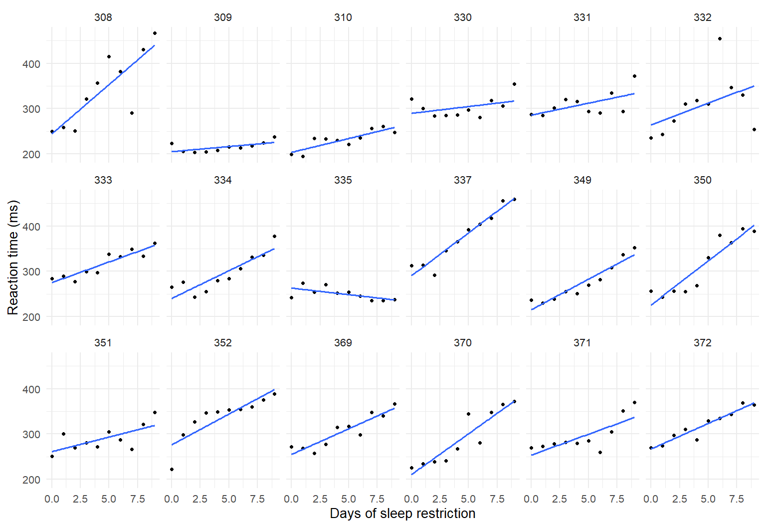
Figure 10.1 shows each person’s reaction times, with their own trend line.
ggplot(sleepstudy, aes(x = Days, y = Reaction)) +geom_point(size =1) +geom_smooth(method ="lm", se =FALSE, linewidth =0.7) +facet_wrap(~ Subject, ncol =6) +labs(x ="Days of sleep restriction", y ="Reaction time (ms)") +theme_minimal(base_size =10)
Figure 10.1: Reaction times over 10 days of sleep restriction, one panel per person, with each person’s own trend line.
Two things are clear. Almost everyone gets slower as the days go by. And people differ: some start faster than others (different intercepts), and some slow down more than others (different slopes).
10.2.1 Random intercepts
An ordinary regression would fit one line through all 180 points, as if they came from 180 different people. A random intercept model fits one average line, but lets each person have their own starting level. In the formula, (1 | Subject) means “a separate intercept for each subject”, and lmer() fits the model:
sleep_ri <-lmer(Reaction ~ Days + (1| Subject), data = sleepstudy)summary(sleep_ri)
Linear mixed model fit by REML ['lmerMod']
Formula: Reaction ~ Days + (1 | Subject)
   Data: sleepstudy

REML criterion at convergence: 1786.5

Scaled residuals:
    Min      1Q  Median      3Q     Max
-3.2257 -0.5529  0.0109  0.5188  4.2506

Random effects:
 Groups   Name        Variance Std.Dev.
 Subject  (Intercept) 1378.2   37.12
 Residual              960.5   30.99
Number of obs: 180, groups:  Subject, 18

Fixed effects:
            Estimate Std. Error t value
(Intercept) 251.4051     9.7467   25.79
Days         10.4673     0.8042   13.02

Correlation of Fixed Effects:
     (Intr)
Days -0.371
The output has two important parts. The fixed effects describe the average line, as in ordinary regression: on day 0, the average reaction time is about 251 ms, and each day of sleep restriction adds about 10.5 ms. The random effects describe how much people vary around the average line. The standard deviation of the intercepts, about 37 ms, says that people’s starting levels typically differ from the average by that much; the residual standard deviation, about 31 ms, is the day-to-day variation within a person.
10.2.2 The intraclass correlation
The random intercept model splits the variation in reaction times into two parts: stable differences between people, and variation within each person from day to day. The intraclass correlation (ICC) compares them:
\[
\text{ICC} = \frac{\text{variance between groups}}{\text{variance between groups} + \text{variance within groups}}
\]
About 59% of the variation in reaction times is due to stable differences between people. The ICC can be read as a comparison of how much people differ from each other with how much each person varies. An ICC of 0 would mean the grouping does not matter: two measurements of the same person are no more alike than measurements of two different people. The higher the ICC, the more the measurements of one person repeat each other, and the more wrong an ordinary regression would be.
10.2.3 Random slopes
The random intercept model still assumes that everyone slows down at the same rate, which Figure 10.1 shows is not true. A random slope model lets each person have their own slope as well. In the formula, (Days | Subject) means “a separate intercept and slope of Days for each subject”:
sleep_rs <-lmer(Reaction ~ Days + (Days | Subject), data = sleepstudy)summary(sleep_rs)$coefficients
             Estimate Std. Error   t value
(Intercept) 251.40510   6.824597 36.838090
Days         10.46729   1.545790  6.771481
VarCorr(sleep_rs)
 Groups   Name        Std.Dev. Corr
 Subject  (Intercept) 24.7407
          Days         5.9221  0.066
 Residual             25.5918
The average effect of a day of sleep restriction is the same, about 10.5 ms, but its standard error has grown from 0.8 to 1.55. People’s slopes vary with a standard deviation of about 5.9 ms per day, so for most people a day of sleep restriction adds somewhere between about 5 and 16 ms. Ignoring that variation made the random intercept model too confident about the average.
A likelihood ratio test, run with anova(), shows whether the random slope is worth adding:
The p-value is tiny: the random slopes improve the model clearly. The AIC column agrees. AIC balances fit against complexity, and lower is better.
10.3 Change in wellbeing over two years
The wellbeing study has up to four semester records for each student, joined with their background information. The variable time counts semesters from the first, so that time 0 is semester 1:
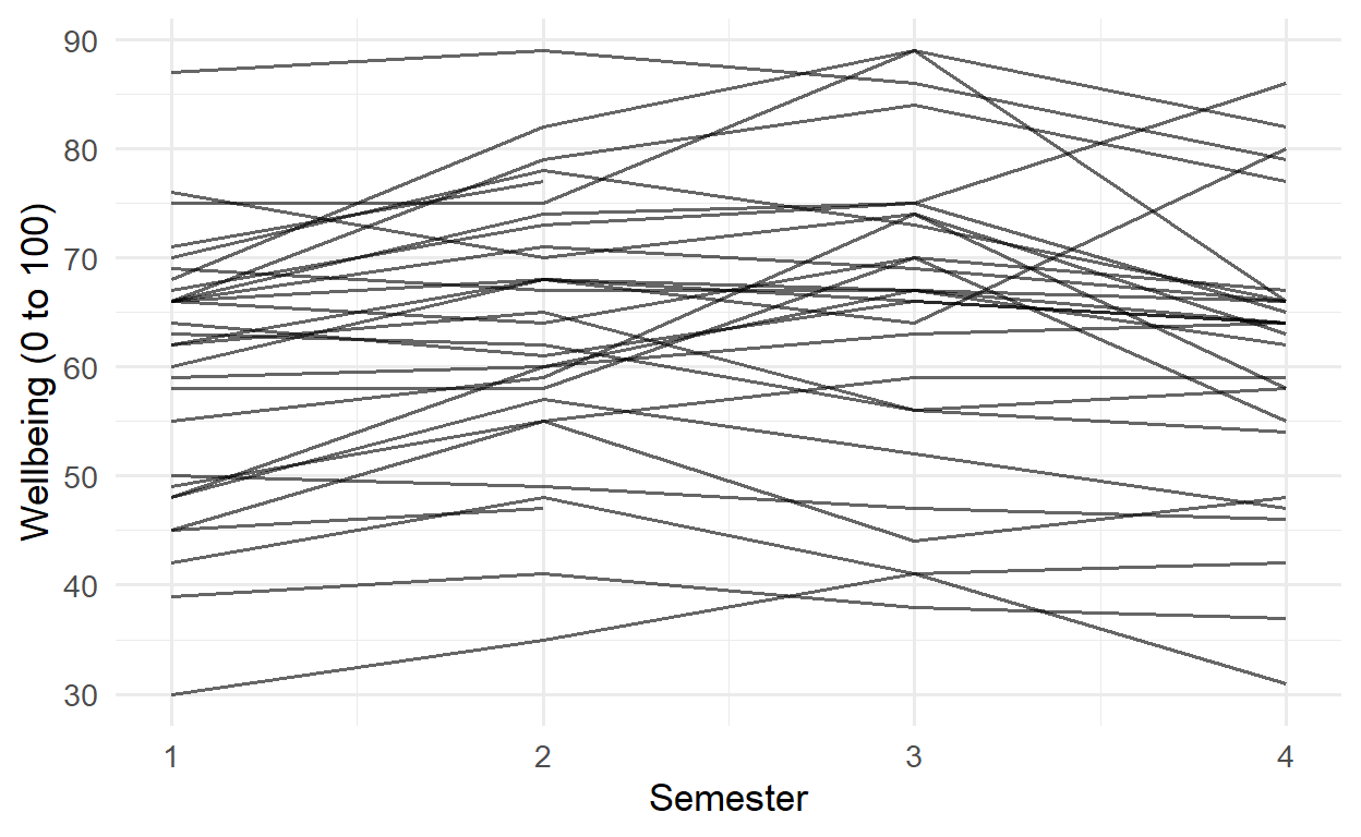
Figure 10.2 shows the wellbeing of 30 randomly chosen students across the four semesters.
set.seed(9)some_students <-sample(unique(panel$student_id), 30)panel |>filter(student_id %in% some_students) |>ggplot(aes(x = semester, y = wellbeing, group = student_id)) +geom_line(alpha =0.6) +labs(x ="Semester", y ="Wellbeing (0 to 100)") +theme_minimal(base_size =13)
Figure 10.2: Wellbeing over four semesters for 30 randomly chosen students.
Students differ enormously in their overall level, much more than any student changes from one semester to the next. A model with no predictors, only a random intercept for each student, puts a number on this through the ICC:
wb_null <-lmer(wellbeing ~1+ (1| student_id), data = panel)vc_null <-as.data.frame(VarCorr(wb_null))vc_null$vcov[1] /sum(vc_null$vcov)
[1] 0.7809117
About 78% of all the variation in wellbeing is between students: students differ from each other far more than they change. The consequence for the amount of information in the data can be calculated. The design effect, \(1 + (m - 1) \times \text{ICC}\), where \(m\) is the number of records per student, says how many times more records are needed to give the same information as independent observations:
               records          design_effect independent_equivalent
           2326.000000               3.246423             716.480955
The 2326 semester records carry about as much information about average wellbeing as 716 independent observations would. Treating them as 2326 independent records would therefore be seriously wrong.
10.3.1 Why ordinary regression misleads
The first question about change is whether wellbeing declines over time. The wrong way to answer it is an ordinary regression that ignores the structure:
summary(lm(wellbeing ~ time, data = panel))$coefficients
              Estimate Std. Error    t value   Pr(>|t|)
(Intercept) 61.6319636  0.4124650 149.423511 0.00000000
time        -0.3794867  0.2235408  -1.697618 0.08971384
The slope is slightly negative, but not significant. The mixed model, with a random intercept and slope for each student, gives a different result:
wb_growth <-lmer(wellbeing ~ time + (time | student_id), data = panel)summary(wb_growth)$coefficients
              Estimate Std. Error    t value
(Intercept) 61.6455545  0.4764479 129.385717
time        -0.4342392  0.1107653  -3.920355
The average slope is similar, about -0.43 points per semester, but its standard error has fallen from 0.22 to 0.11, and the decline is now clearly significant (a t value of about -3.9). The reason is that the ordinary regression lumps the large, stable differences between students into its error term, which drowns the small change within each student. The mixed model separates the two, and sees the change clearly.
In the simulation at the start of the chapter, ignoring the structure made a non-existent effect look significant; in the sleep study, ignoring the differences in slopes made the average look more certain than it was; here, ignoring the structure makes a real decline look uncertain. The direction of the error depends on the data, but the error is always there.
10.3.2 Confidence intervals and p-values
The lme4 package deliberately prints no p-values for fixed effects, because calculating them exactly for mixed models is not straightforward. There are three common solutions. The first is to report confidence intervals, which are often more informative than p-values anyway. The function confint() calculates them, and method = "Wald" is quick:
confint(wb_growth, parm ="beta_", method ="Wald")
                 2.5 %     97.5 %
(Intercept) 60.7117337 62.5793752
time        -0.6513351 -0.2171432
The argument parm = "beta_" asks for the fixed effects only. The interval for time lies entirely below zero: wellbeing declines.
The second solution is a likelihood ratio test, comparing models with and without a term with anova(), as for the random slopes above. The third is the lmerTest package, which adds p-values to the summary() output and is used in most published research. Once it is loaded, lmer() models fitted afterwards include a p-value for each fixed effect:
library(lmerTest)wb_growth_p <-lmer(wellbeing ~ time + (time | student_id), data = panel)summary(wb_growth_p)$coefficients
              Estimate Std. Error       df    t value     Pr(>|t|)
(Intercept) 61.6455545  0.4764479 598.9342 129.385717 0.000000e+00
time        -0.4342392  0.1107653 571.4997  -3.920355 9.914491e-05
The new columns are the degrees of freedom (estimated by Satterthwaite’s method) and the p-value, Pr(>|t|). The decline over time is clearly significant, in agreement with the confidence interval. Chapter 5’s hypothesis for RQ8, that wellbeing declines over the two years, is supported.
10.3.3 Persistence of the workshop effect
Chapter 7 showed that the workshop raised wellbeing in semester 2. A mixed model can compare the two groups in every semester at once, using every record, including the first year of the students who later left. Treating semester as a factor lets each semester have its own average, and the interaction with workshop lets the gap between the groups differ from semester to semester:
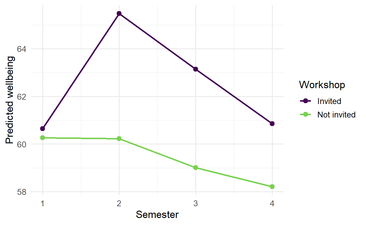
The coefficients are easier to understand as predicted averages. The function predict() with re.form = NA gives the predictions for the average student, ignoring the random effects:
Figure 10.3: Predicted wellbeing in each semester by workshop group, from the mixed-effects model.
The gap between the groups is 0.4 points in semester 1, before the workshop, 5.2 in semester 2, 4.1 in semester 3, and 2.6 in semester 4. The workshop’s effect is real, but it fades over the following year. For the thesis’s recommendations, that matters: a short follow-up session each year might keep the benefit going.
The interaction coefficients test whether the gap in each semester differs from the gap in semester 1. All three do (the largest p-value is 0.001).
10.3.4 Change in GPA
The same growth model can be fitted to GPA:
gpa_growth <-lmer(gpa ~ time + (time | student_id), data = panel)
boundary (singular) fit: see help('isSingular')
R warns that the fit is singular. This message is common, and worth understanding. It means the model is more complex than the data supports: here, the students’ GPA slopes hardly vary at all, so the model cannot estimate their spread. The solution is to simplify, keeping only the random intercept:
gpa_growth <-lmer(gpa ~ time + (1| student_id), data = panel)summary(gpa_growth)$coefficients
                 Estimate  Std. Error        df     t value  Pr(>|t|)
(Intercept)  3.0921628374 0.013015341  806.5702 237.5783101 0.0000000
time        -0.0004749256 0.003392086 1738.6474  -0.1400099 0.8886684
The slope of time is almost exactly zero: grades stay stable over the two years, even though wellbeing falls. A non-change is a finding too, and here an interesting one.
10.4 Students within supervisors
The students are also nested within supervisors, and a model can include random intercepts for both levels at once:
wb_levels <-lmer(wellbeing ~ time + (1| supervisor_id) + (1| student_id), data = panel)VarCorr(wb_levels)
 Groups        Name        Std.Dev.
 student_id    (Intercept) 9.7748
 supervisor_id (Intercept) 4.4098
 Residual                  5.6189
Because every student ID is unique, R knows that students are nested within supervisors. Dividing each variance by the total shows where the variation lies:
About 13% of all the variation in wellbeing lies between supervisors: students of the same supervisor are noticeably more alike. Most of the variation, 65%, lies between students within the same supervisor, and the remaining 22% is change within students from semester to semester. For the university, the supervisor share is a practical finding: who supervises a student makes a measurable difference to their wellbeing. It also means that any comparison of supervisors, or of anything assigned to supervisors, must allow for this grouping, as the simulation at the start of the chapter showed.
10.5 Counts and yes-or-no outcomes
Like ordinary regression, mixed models extend to other kinds of outcome. The function glmer() fits a generalised linear mixed model: family = binomial for yes-or-no outcomes, as in Chapter 8’s logistic regression, and family = poisson for counts, such as the number of meetings a student had with their supervisor each semester.
The model below examines whether students who feel more supported meet their supervisor more often. Support is calculated from the questionnaire, as before:
               Estimate Std. Error    z value     Pr(>|z|)
(Intercept)  0.06224346 0.07134373  0.8724446 3.829659e-01
support      0.39258255 0.01975713 19.8704237 7.338090e-88
programmePhD 0.17676057 0.02881998  6.1332638 8.609423e-10
Poisson coefficients are on a log scale, and exp() turns them into rate ratios:
exp(fixef(meetings_model))
 (Intercept)      support programmePhD
    1.064221     1.480800     1.193345
Each extra point of support goes with about 48% more meetings per semester, and PhD students have about 19% more meetings than Master’s students, holding support constant. As always with observational data, the direction is not certain: more meetings may also make students feel more supported.
NoteMissing data and mixed models
Chapter 6 found that the students who left after the first year were not a random group. Mixed models handle this better than most methods: they use every record each student provided, including the first year of those who left, instead of dropping those students entirely. The results remain trustworthy as long as leaving depends on things the model can see, such as the students’ earlier wellbeing, which is the “missing at random” situation of Chapter 6.
10.6 Reporting a mixed-effects model
A mixed-effects model is reported with both of its parts: the fixed effects, with confidence intervals, and the random effects, as standard deviations or variance shares. The report should also say how many observations and groups the model used, and which random effects it included.
TipWriting it up
A linear mixed-effects model with random intercepts and slopes for students (2326 observations of 600 students) showed that wellbeing declined slightly over the four semesters, by 0.43 points per semester (95% CI [0.22, 0.65]). Students differed considerably in their overall wellbeing (SD of intercepts = 10.7); 78% of the variation in wellbeing was between students.
NoteIn your field: agriculture
R’s ChickWeight data records the weight of 50 chicks, measured every few days from birth to 21 days old, on one of four diets. It has exactly the structure of the wellbeing data: repeated measurements of the same individuals, in groups. A random-slope model compares how fast chicks grow on each diet:
chick_model <-lmer(weight ~ Time * Diet + (Time | Chick), data = ChickWeight)round(summary(chick_model)$coefficients, 2)
Chicks on diet 1 gain about 6.3 grams a day. The interaction terms show how much faster chicks grow on the other diets: diet 3 adds about 5.1 grams a day, which is 82% more than the rate on diet 1.
10.7 Common misconceptions
Mixed models are powerful, and several misunderstandings about grouped data survive even among experienced researchers.
“More rows means more evidence.” Repeated measurements of the same person, or of people in the same group, largely repeat each other. The design effect shows how much less information they carry.
“Ignoring the grouping only makes results a little less precise.” It can produce false alarms many times more often than intended, as the simulation showed, or hide real effects.
“Averaging each person’s records solves the problem.” It removes the dependence, but throws away the information about change, and gives unequal weight to people with different numbers of records.
“A singular fit means the model is wrong.” It means the model is more complex than the data can support; simplifying the random effects is usually enough.
10.8 Chapter review
10.8.1 Summary
Repeated measures and nested data break the independence assumption of ordinary regression, which then gets the uncertainty wrong, in either direction. A simulation shows false alarms far above 5% when grouping is ignored.
Mixed-effects models have fixed effects (the average relationships) and random effects (how groups vary around them). (1 | group) gives each group its own intercept; (x | group) also its own slope of x.
The intraclass correlation is the share of variation between groups: how much groups differ from each other compared with how much members vary within them. The design effect shows how much less information grouped records carry.
lme4 prints no p-values: use confidence intervals, likelihood ratio tests with anova(), or the lmerTest package.
Interactions with time show whether an effect grows or fades. predict(..., re.form = NA) gives predictions for the average case.
A singular fit means the model is too complex for the data: simplify the random effects.
glmer() fits mixed models for yes-or-no outcomes (binomial) and counts (poisson; exp() of the coefficients gives rate ratios).
Mixed models use all available records, which helps when participants drop out.
10.8.2 Key terms
Repeated measures, nested data, mixed-effects model, multilevel model, fixed effect, random effect, random intercept, random slope, intraclass correlation, design effect, likelihood ratio test, AIC, singular fit, generalised linear mixed model, Poisson model, count outcome, rate ratio.
10.9 Exercises
The playground has these and more, with hints and solutions.
Fit a random intercept model for sleep_hours over time (sleep_hours ~ time + (1 | student_id)). Calculate the ICC, and describe whether sleep changes over the semesters.
Add a random slope of time to the model in Exercise 1, and compare the two models with anova(). Decide whether the random slope is worth keeping.
Fit wellbeing ~ time * study_mode + (time | student_id), and describe whether part-time students’ wellbeing changes at a different rate.
Fit a model with random intercepts for supervisors and students for study_hours, and calculate how much of its variation lies between supervisors.
Change the simulation at the start of the chapter so that supervisors differ more (sd = 10 for style). Describe what happens to the false alarm rate of the ordinary regression, and explain why.
In your own words, explain to a fellow student why an ordinary regression of all the semester records would be wrong.
10.10 Further reading
Data Analysis Using Regression and Multilevel/Hierarchical Models(Gelman and Hill 2007) is a classic, readable introduction to multilevel models.
“Fitting Linear Mixed-Effects Models Using lme4” (Bates et al. 2015) describes the lme4 package and its formula syntax in detail.
References
Bates, Douglas, Martin Mächler, Ben Bolker, and Steve Walker. 2015. “Fitting Linear Mixed-Effects Models Using lme4.”Journal of Statistical Software 67 (1): 1–48. https://doi.org/10.18637/jss.v067.i01.
Belenky, Gregory, Nancy J. Wesensten, David R. Thorne, et al. 2003. “Patterns of Performance Degradation and Restoration During Sleep Restriction and Subsequent Recovery: A Sleep Dose-Response Study.”Journal of Sleep Research 12 (1): 1–12. https://doi.org/10.1046/j.1365-2869.2003.00337.x.
Gelman, Andrew, and Jennifer Hill. 2007. Data Analysis Using Regression and Multilevel/Hierarchical Models. Cambridge University Press. https://doi.org/10.1017/CBO9780511790942.