14 Advanced Clustering

Every clustering method carries a definition of what a group is, usually without saying so. One definition says that a group is a set of cases close to a common centre. Another says that a group is a population with its own distribution, so that cases between groups can belong partly to each. A third says that a group is a dense region of data, separated from other groups by sparse regions, which leaves room for cases that belong to no group at all. The definition chosen decides what the method can find, and a clustering is only as meaningful as the definition behind it.

Chapter 9 used k-means, which takes the first definition. It divided the students of the wellbeing study into four lifestyle profiles, but left open questions that any examiner might ask: how sure one can be about which profile a student belongs to, whether four is really the right number, and whether some students fit no profile. This chapter addresses them with two methods that relax the assumptions of k-means. Gaussian mixture models give each student a probability of belonging to each profile, and choose the number of profiles with a statistical criterion. DBSCAN defines clusters as dense regions of data, and labels students in sparse regions as noise: people who fit no group. The chapter ends with the question behind all clustering: how to judge whether a clustering is any good.

TipBy the end of this chapter you will be able to

• Explain three definitions of a group, and the limitations of k-means: hard assignments, round clusters, and no room for outliers.
• Fit a Gaussian mixture model with mclust, choose the number of clusters with BIC, and interpret membership probabilities.
• Find dense clusters and noise points with DBSCAN, and choose its settings.
• Evaluate a clustering with the silhouette, agreement between methods (the adjusted Rand index), and interpretability.

Teaching & Practice: Interactive Lecture Slides · Browser Playground Exercises

14.1 The profile data

The data is exactly that of Chapter 9: each student’s average sleep, study hours, caffeine, and exercise across the semesters, and their stress, support, and satisfaction scores, scaled to z-scores.

library(dplyr)
library(ggplot2)

q <- questionnaire
q$stress_4 <- 6 - q$stress_4

scores <- q |>
  mutate(
    stress       = rowMeans(pick(stress_1:stress_6), na.rm = TRUE),
    support      = rowMeans(pick(support_1:support_6), na.rm = TRUE),
    satisfaction = rowMeans(pick(satisfaction_1:satisfaction_4), na.rm = TRUE)
  ) |>
  select(student_id, stress, support, satisfaction)

profiles <- semesters |>
  summarise(across(c(sleep_hours, study_hours, caffeine_mg, exercise_days),
                   ~ mean(.x, na.rm = TRUE)),
            .by = student_id) |>
  left_join(scores, join_by(student_id)) |>
  na.omit()

profile_data <- scale(profiles |> select(-student_id))

set.seed(123)
kmeans_clusters <- kmeans(profile_data, centers = 4, nstart = 25)

The last two lines repeat Chapter 9’s k-means solution, for comparison.

14.2 What counts as a group

k-means is simple and fast, but its definition of a group brings three strong assumptions. It assumes that every case belongs to exactly one cluster, with complete certainty, so a student halfway between two profiles is assigned to one of them as firmly as a student at the centre. It assumes that clusters are round and similar in size: because each case goes to the nearest centre, k-means draws straight boundaries halfway between centres, and elongated or unequal clusters are cut up wrongly. And it assumes that every case belongs to some cluster, with no way to say that a student fits nowhere. Real groups of people rarely satisfy these assumptions.

A simulation shows how much the definition matters. The code below creates data with a known structure: a small round group, a long thin group, and 15 scattered points that belong to neither. It then clusters the data in three ways, with k-means (groups around centres), a Gaussian mixture model (groups as distributions), and DBSCAN (groups as dense regions), the two methods this chapter introduces:

library(mclust)
library(dbscan)

set.seed(8)
shapes <- bind_rows(
  tibble(x = rnorm(100, 0, 0.4), y = rnorm(100, 0, 0.4), truth = "Round group"),
  tibble(x = rnorm(100, 3, 2), y = rnorm(100, 1.4, 0.2), truth = "Long group"),
  tibble(x = runif(15, -2, 7), y = runif(15, -2, 4), truth = "Scattered")
)
xy <- shapes |> select(x, y)

shape_clusters <- bind_rows(
  shapes |> mutate(method = "k-means", cluster = factor(kmeans(xy, 2, nstart = 25)$cluster)),
  shapes |> mutate(method = "Mixture model", cluster = factor(Mclust(xy, G = 2, verbose = FALSE)$classification)),
  shapes |> mutate(method = "DBSCAN", cluster = factor(dbscan(xy, eps = 0.5, minPts = 5)$cluster))
) |>
  mutate(method = factor(method, levels = c("k-means", "Mixture model", "DBSCAN")),
         cluster = forcats::fct_recode(cluster, noise = "0"))

ggplot(shape_clusters, aes(x, y, colour = cluster)) +
  geom_point(size = 1.2) +
  facet_wrap(~ method) +
  scale_colour_manual(values = c("1" = "#2f6793", "2" = "#e07b39", "3" = "#36a269",
                                 "4" = "#8b68b5", noise = "grey65")) +
  coord_equal() +
  theme_minimal(base_size = 11)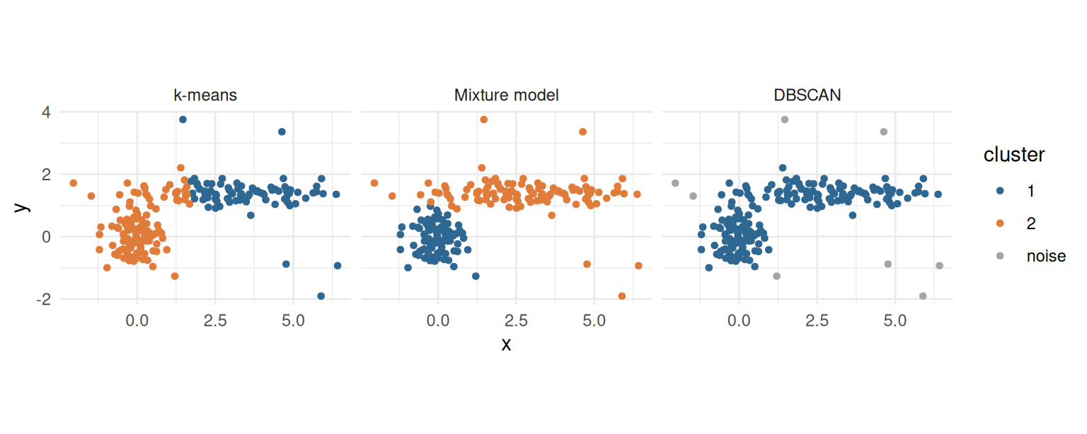

Figure 14.1: The same simulated data clustered by k-means, a Gaussian mixture model, and DBSCAN. The data contains a round group, a long thin group, and scattered points that belong to neither; each method’s definition of a group decides what it finds.

The three methods see different groups in the same data. Their agreement with the two real groups can be measured with the adjusted Rand index, introduced at the end of the chapter, where 1 means perfect agreement and 0 means no more than chance. k-means scores 0.53: looking for round groups around two centres, it draws a straight boundary through the long group and gives its left end to the round group. The mixture model scores 0.98, because it allows the long group its elongated shape. DBSCAN scores 0.00, for a different reason: the end of the long group touches the round group, so the two form one continuous dense region, and by DBSCAN’s definition that is one group. DBSCAN is, however, the only method that can say that points belong to no group: it labels 6 of the 15 scattered points as noise, while the other two methods must place every one of them in a group. No method is right in general. Each is right for data whose groups match its definition, which is why the definition should be chosen deliberately, and stated.

14.3 Gaussian mixture models

A Gaussian mixture model (GMM) assumes that the data comes from a mix of several groups, each with its own normal (Gaussian) distribution, and estimates each group’s centre, spread, and size from the data.

14.3.1 A one-variable example

The idea is easiest to see with one variable. R’s faithful data records the waiting time, in minutes, between 272 eruptions of the Old Faithful geyser in Yellowstone National Park. The histogram in Figure 14.2 has two humps: short waits and long waits. The mclust package fits a mixture model with Mclust():

geyser <- Mclust(faithful$waiting)
summary(geyser, parameters = TRUE)

---------------------------------------------------- 
Gaussian finite mixture model fitted by EM algorithm 
---------------------------------------------------- 

Mclust E (univariate, equal variance) model with 2 components: 

 log-likelihood   n df       BIC       ICL
      -1034.002 272  4 -2090.427 -2099.576

Clustering table:
  1   2 
 99 173 

Mixing probabilities:
        1         2 
0.3609461 0.6390539 

Means:
       1        2 
54.61675 80.09239 

Variances:
       1        2 
34.44093 34.44093 

The function tried mixtures of one to nine groups and chose 2. The output describes them: the mixing probabilities are the sizes of the groups (about 36% and 64% of eruptions), the means are their centres (about 55 and 80 minutes), and the variances their spreads. Figure 14.2 draws the two fitted normal curves over the data.

Figure 14.2: Waiting times between eruptions of Old Faithful, with the two normal distributions of the fitted mixture model.

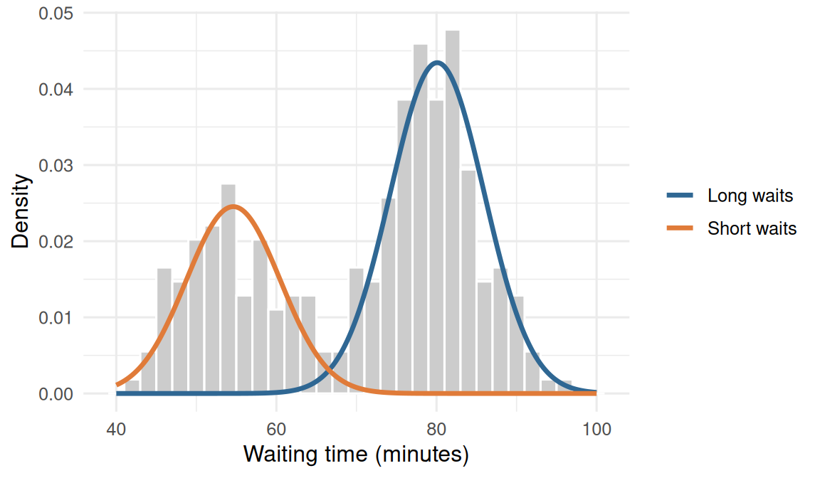
The key difference from k-means appears between the groups. A waiting time of 67 minutes lies between them. Instead of forcing it into one, the model gives the probability that it came from each:

predict(geyser, newdata = c(50, 67, 85))$z |> round(2)

        1    2
[1,] 1.00 0.00
[2,] 0.42 0.58
[3,] 0.00 1.00

A wait of 50 minutes almost certainly belongs to the short group, and 85 minutes to the long group, but 67 minutes is uncertain. These membership probabilities (also called soft assignments) are the main advantage of mixture models: they say not just which group a case is in, but how sure that is.

14.3.2 Choosing the number of clusters with BIC

With more variables, each group is described by a centre and a covariance matrix, which sets its shape: round or elongated, and tilted in any direction. Groups can be allowed to differ in size (volume), shape, and orientation, or forced to be the same. mclust names each combination with three letters, such as EEE (all equal) or VVV (all variable), and fits them all for each number of groups.

To choose among them, it uses the Bayesian information criterion (BIC). BIC rewards a model for fitting the data well and penalises it for every parameter it needs, so a more complex model must earn its extra parameters. In mclust, higher BIC is better. For the profile data:

set.seed(123)
profile_gmm <- Mclust(profile_data, G = 1:8)
summary(profile_gmm)

---------------------------------------------------- 
Gaussian finite mixture model fitted by EM algorithm 
---------------------------------------------------- 

Mclust EVE (ellipsoidal, equal volume and orientation) model with 3 components: 

 log-likelihood   n df       BIC       ICL
      -5128.189 599 63 -10659.28 -10752.69

Clustering table:
  1   2   3 
231 174 194 

library(factoextra)
fviz_mclust(profile_gmm, what = "BIC")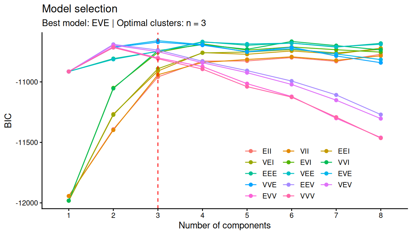

Figure 14.3: BIC for Gaussian mixture models with one to eight clusters. Each line is one covariance structure; higher is better.

BIC chooses 3 clusters with the EVE structure (ellipsoidal clusters of equal size and orientation, but different shapes). The best four-cluster model is about 8.7 BIC points behind. A common rule of thumb reads a BIC difference above 6 as strong evidence and above 10 as very strong, so the data favours three profiles, although four remain a reasonable alternative (exercise 1 explores them).

14.3.3 Describing the profiles

As in Chapter 9, a cluster means something only once it is described:

profiles <- profiles |>
  mutate(gmm_cluster = profile_gmm$classification)

profiles |>
  summarise(students = n(), across(sleep_hours:satisfaction, ~ round(mean(.x), 1)),
            .by = gmm_cluster) |>
  arrange(gmm_cluster)

  gmm_cluster students sleep_hours study_hours caffeine_mg exercise_days stress
1           1      231         6.7        17.9       151.7           2.2    3.3
2           2      174         7.2        25.0       126.2           3.7    2.6
3           3      194         5.5        41.7       284.1           1.3    3.6
  support satisfaction
1     2.8          2.7
2     3.6          3.9
3     3.3          3.1

The three profiles are clear. One is balanced: the most sleep and exercise, the least stress, and the highest support and satisfaction. One is overloaded: long study weeks, short sleep, a lot of caffeine, little exercise, and the most stress. The third, the largest, combines few study hours with low support and low satisfaction: students who seem disengaged or isolated. The cluster numbers are arbitrary labels. A cross-table compares the solution with k-means:

table(gmm = profile_gmm$classification, kmeans = kmeans_clusters$cluster)

   kmeans
gmm   1   2   3   4
  1   5 191  34   1
  2   0   3 166   5
  3  80   3   0 111

The mixture model’s three profiles correspond closely to Chapter 9’s four k-means clusters: the balanced and disengaged groups largely match, and the two k-means “overloaded” clusters, one of them with very high caffeine, are joined into one. The mixture model, with its more flexible cluster shapes, did not need to split the overloaded students in two.

14.3.4 Certainty of assignment

The matrix profile_gmm$z holds each student’s membership probabilities, one column per cluster, and profile_gmm$uncertainty is 1 minus the largest of them.

head(round(profile_gmm$z, 2))

  [,1] [,2] [,3]
1 0.63 0.37    0
2 0.99 0.00    0
3 0.14 0.86    0
4 0.00 0.00    1
5 0.10 0.90    0
6 1.00 0.00    0

certainty <- apply(profile_gmm$z, 1, max)
sum(certainty < 0.8)

[1] 79

The call apply(..., 1, max) takes the maximum of each row. Most students belong clearly to one profile, but 79 have less than an 80% probability for their most likely profile. Figure 14.4 shows where they are.

fviz_mclust(profile_gmm, what = "uncertainty")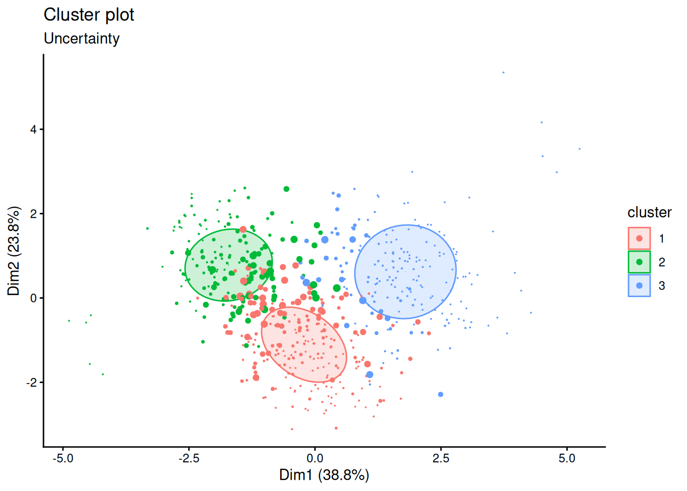

Figure 14.4: The three mixture model clusters on the first two principal components. Larger points are students whose profile is more uncertain.

The uncertain students lie where the profiles meet. For a thesis, this is honest and useful: instead of claiming that every student has one profile, it can report the share of students who clearly fit a profile, and treat the rest as mixtures. A later analysis could use the probabilities themselves, for example as weights, rather than the hard labels.

14.4 Clusters as dense regions

DBSCAN (density-based spatial clustering of applications with noise) takes a different view. A cluster is a region where cases are packed closely together, separated from other clusters by sparser regions. Cases in sparse regions belong to no cluster; they are noise. DBSCAN does not need the number of clusters in advance, can find clusters of any shape, and can say “this case fits nowhere”.

It needs two settings: eps (epsilon), the radius of the neighbourhood around each case, and minPts, the number of cases a neighbourhood must contain for the case to be at the heart of a cluster. A case with at least minPts cases within eps is a core point. Core points within eps of each other are joined into the same cluster, and cases near a core point are added to its cluster as border points. Everything else is noise.

14.4.1 A small example

Twelve points show how it works: two tight groups of five, and two isolated points.

tiny <- tibble(
  x = c(1.0, 1.2, 1.1, 0.9, 1.3,   4.0, 4.2, 3.9, 4.1, 4.3,   2.5, 5.5),
  y = c(1.0, 1.1, 1.3, 1.2, 0.9,   3.0, 3.2, 3.1, 2.8, 3.0,   4.5, 0.5)
)

tiny_db <- dbscan(tiny, eps = 0.5, minPts = 3)
tiny_db$cluster

 [1] 1 1 1 1 1 2 2 2 2 2 0 0

The two tight groups become clusters 1 and 2, and the two isolated points are labelled 0: noise. k-means with two clusters would have had to put the isolated points into one of the groups.

14.4.2 Choosing eps

The result depends heavily on eps. A common guide is the k-nearest-neighbour distance plot: for each case, the distance to its \(k\)-th nearest neighbour, sorted from smallest to largest. Most cases have close neighbours; the curve bends sharply upwards where the isolated cases begin, and that bend suggests a value for eps. With minPts set to 8, a common choice for data with seven variables (about the number of variables plus one or more), the plot uses \(k = 7\):

kNNdistplot(profile_data, k = 7)
abline(h = 2, lty = "dashed")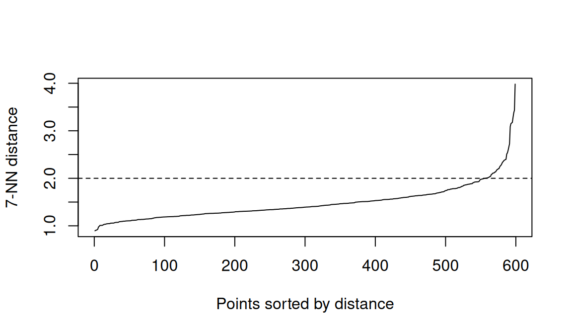

Figure 14.5: Distance from each student to their seventh-nearest neighbour, sorted. The dashed line marks eps = 2.

The curve bends at a distance of about 2, so eps = 2 is used:

profile_db <- dbscan(profile_data, eps = 2, minPts = 8)
profile_db

DBSCAN clustering for 599 objects.
Parameters: eps = 2, minPts = 8
Using euclidean distances and borderpoints = TRUE
The clustering contains 1 cluster(s) and 13 noise points.

  0   1 
 13 586 

Available fields: cluster, eps, minPts, metric, borderPoints

DBSCAN finds 1 cluster and 13 noise points. At first this looks like a failure: no profiles at all. But it is an informative result. DBSCAN looks for dense regions separated by gaps, and the students form one continuous cloud, in which the profiles found by k-means and the mixture model overlap without gaps between them. (Smaller values of eps break the cloud into fragments and label hundreds of students as noise; try it in the exercises.) The profiles are real differences in where students sit in the cloud, not separate islands.

14.4.3 Students who fit no profile

The noise points answer the last of the open questions: whether some students fit no profile. Their values are:

profiles |>
  filter(profile_db$cluster == 0) |>
  select(sleep_hours:satisfaction) |>
  round(1)

   sleep_hours study_hours caffeine_mg exercise_days stress support
1          3.6        60.5       772.5           0.5    3.2     4.0
2          4.6        45.8       592.5           2.5    2.8     2.7
3          9.7         2.2        26.2           5.2    1.7     2.7
4          3.7        61.5       842.5           0.0    3.5     3.7
5          9.4         5.5        23.8           6.2    2.7     3.7
6          3.8        63.0       780.0           0.5    2.0     3.5
7          3.7        63.2       742.5           0.0    1.8     4.3
8          9.6         4.2        21.2           5.0    2.7     3.5
9          9.8         5.2        18.8           5.8    2.6     2.2
10         9.5         2.0        20.0           6.2    2.5     2.5
11         4.0        65.5       735.0           0.5    3.2     3.3
12         4.4        30.2       703.8           0.8    3.2     4.6
13         3.8        35.8       641.2           1.0    3.0     1.8
   satisfaction
1           4.2
2           4.0
3           4.2
4           3.8
5           3.7
6           2.8
7           4.7
8           4.2
9           3.5
10          3.5
11          3.2
12          3.0
13          2.8

Two kinds of unusual student stand out. Among the noise points, 5 students study around 60 hours a week, sleep about 4 hours a night or less, drink over 700 mg of caffeine a day (about seven cups of coffee), and hardly exercise: more extreme than anyone in the overloaded profile. 5 others are the opposite: close to 10 hours of sleep, very few study hours, very little caffeine, and exercise almost every day. The remaining few are extreme versions of the overloaded profile. In Chapter 6, extreme values were checked one variable at a time; DBSCAN finds students who are unusual in their combination of values.

These students should not be deleted: they are real students, and the extreme workers are exactly the students a wellbeing service would want to know about. They are reported separately, as students who do not fit the profiles, and the profiles are checked for whether they change when these students are left out.

14.5 Evaluating a clustering

In supervised learning, a model is judged against the true answers. In clustering there are usually no true answers, so evaluation rests on several kinds of evidence, none decisive on its own.

Internal measures judge how compact and well separated the clusters are, using the data alone. The silhouette of Chapter 9 is the most common, and BIC plays this role for mixture models. The silhouette() function from the cluster package calculates it for any clustering:

library(cluster)
profile_distances <- dist(profile_data)

mean(silhouette(kmeans_clusters$cluster, profile_distances)[, "sil_width"])

[1] 0.2135627

mean(silhouette(profile_gmm$classification, profile_distances)[, "sil_width"])

[1] 0.2272005

Both averages are low (the silhouette runs from −1 to 1), which confirms what DBSCAN suggested: the profiles overlap, and no clustering of this data will be crisp.

Agreement between methods asks whether different reasonable methods find similar groups. The adjusted Rand index (ARI) measures the agreement between two clusterings. It counts the pairs of cases that both clusterings put together or both put apart, and adjusts for the agreement expected by chance: 1 means identical groupings (whatever the labels), and 0 means no more agreement than chance. A tiny example shows that the labels themselves do not matter:

first  <- c(1, 1, 1, 2, 2, 2)
second <- c("B", "B", "B", "A", "A", "A")
third  <- c(1, 1, 2, 2, 3, 3)
adjustedRandIndex(first, second)

[1] 1

adjustedRandIndex(first, third)

[1] 0.2424242

The first two clusterings group the six people identically, so their ARI is 1, even though the labels differ. The third splits them differently, so its ARI is much lower. For the two methods applied to the profile data:

adjustedRandIndex(kmeans_clusters$cluster, profile_gmm$classification)

[1] 0.6534227

An ARI of 0.65: substantial agreement, especially given that one solution has four clusters and the other three.

External validation compares clusters with known categories, also using the ARI. It is only possible when such categories exist, for example when clustering flowers of known species to test a method. For real profiles there is no answer key, which is exactly why they are being sought.

Stability asks whether the clusters survive small changes: a different random start, a bootstrap sample of the students, or leaving out the unusual students. Clusters that appear only under one setting should not be reported.

Interpretability and usefulness matter most in the end. The clusters should make sense in the light of theory, and they should differ on outcomes they were not built from, such as GPA or considering dropout. The second point can be checked directly:

profiles |>
  left_join(students |> select(student_id, considering_dropout), join_by(student_id)) |>
  summarise(students = n(),
            considering_dropout = round(mean(considering_dropout == "Yes"), 2),
            .by = gmm_cluster) |>
  arrange(gmm_cluster)

  gmm_cluster students considering_dropout
1           1      231                0.21
2           2      174                0.04
3           3      194                0.17

The profiles differ clearly in how many students consider dropping out, although dropout played no part in finding them. That is good evidence that they capture something real about students’ situations.

ImportantReport the choices, not just the clusters

A clustering depends on choices: which variables, how they are scaled, which method, how many clusters, and settings such as eps. Different reasonable choices can give different answers. In a thesis, report each choice and why it was made, show the evidence for the number of clusters (BIC, silhouette), say how clearly students fit (for example, the share with a membership probability above 0.8), and describe how robust the profiles are to other reasonable choices.

NoteIn your field: earth sciences

DBSCAN was designed for spatial data, where clusters can have any shape. R’s quakes data records the location of 1,000 earthquakes near Fiji since 1964. Plotted on a map, they follow the long, curved lines of two ocean trenches: clusters that are neither round nor of equal size.

quake_db <- dbscan(quakes[, c("long", "lat")], eps = 1.5, minPts = 10)
table(quake_db$cluster)

  0   1   2 
 28 785 187 

quakes |>
  mutate(cluster = factor(quake_db$cluster)) |>
  ggplot(aes(x = long, y = lat, colour = cluster, shape = cluster == "0")) +
  geom_point(alpha = 0.7) +
  scale_colour_manual(values = c("0" = "grey60", "1" = "#2f6793", "2" = "#e07b39")) +
  scale_shape_manual(values = c(`FALSE` = 16, `TRUE` = 4), guide = "none") +
  coord_quickmap() +
  labs(x = "Longitude", y = "Latitude", colour = "Cluster") +
  theme_minimal(base_size = 12)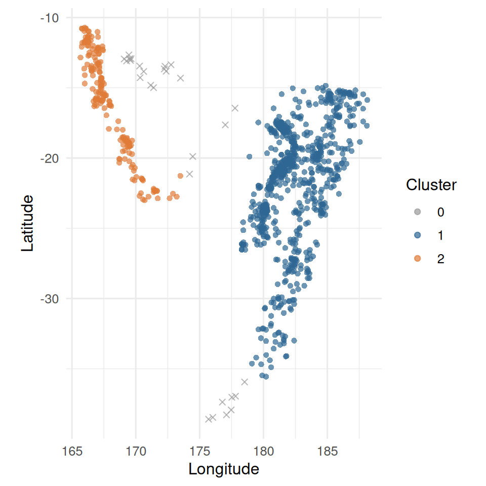

Figure 14.6: Earthquakes near Fiji, clustered by DBSCAN. Grey crosses are noise.

DBSCAN follows the two curved trenches and leaves the scattered earthquakes between and beyond them as noise. Here, unlike in the wellbeing data, there really are dense regions separated by empty space, which is exactly when DBSCAN works best. The function coord_quickmap() gives longitude and latitude the right proportions for a map.

14.6 Common misconceptions

Advanced clustering methods answer some of the weaknesses of k-means, but not the underlying question of whether the groups are real.

• “A more sophisticated method finds the true groups.” Each method finds groups that match its own definition of a group; none can find groups that the data does not contain.
• “Every case belongs to some group.” Cases between groups are better described by membership probabilities, and cases far from all groups by the label “noise”.
• “The best BIC proves the number of groups.” BIC compares models; a model with more groups may be almost as good, and the choice should be reported with its evidence.
• “DBSCAN failed because it found one cluster.” Finding one continuous cloud is itself a finding: the groups found by other methods are regions of that cloud, not separate islands.

14.7 Chapter review

14.7.1 Summary

• Every clustering method has a definition of a group: around a centre (k-means), a distribution (mixture models), or a dense region (DBSCAN). The definition decides what the method can find.
• k-means assigns every case to exactly one round cluster, with no room for uncertainty or outliers.
• A Gaussian mixture model describes the data as a mix of normal distributions of different sizes and shapes. It gives each case a probability of belonging to each cluster, and BIC chooses the number of clusters and their shape (higher is better in mclust).
• On the wellbeing data, the mixture model finds three profiles (balanced, overloaded, and disengaged) that closely match Chapter 9’s k-means clusters, and shows which students fit no profile clearly.
• DBSCAN defines clusters as dense regions and labels cases in sparse regions as noise. It needs eps and minPts; the k-nearest-neighbour distance plot helps choose eps. It works best when clusters are separated by gaps.
• On the wellbeing data, DBSCAN finds one continuous cloud of students and flags a few extreme students who fit no profile.
• Evaluate clusterings with internal measures (silhouette, BIC), agreement between methods (adjusted Rand index), stability, and above all interpretability and relevance to outcomes. Report every choice.

14.7.2 Key terms

Gaussian mixture model, mixture component, mixing probability, membership probability, soft assignment, covariance matrix, Bayesian information criterion (BIC), uncertainty, DBSCAN, density, eps, minPts, core point, border point, noise, k-nearest-neighbour distance plot, internal validation, silhouette, adjusted Rand index, external validation, stability.

14.8 Exercises

The playground has these and more, with hints and solutions.

1. Fit Mclust(profile_data, G = 4) and describe the four profiles. Identify which of the three-cluster profiles has been split, and compare the new solution with Chapter 9’s k-means.
2. Count the students with a membership probability above 0.95 for their profile, and report the share of the sample.
3. Run DBSCAN on the profile data with eps of 1.2, 1.6, and 2.4, describe how the number of clusters and noise points change, and explain why a small eps labels so many students as noise.
4. Leave out the DBSCAN noise students, fit the mixture model again, and describe whether the profiles change.
5. Use adjustedRandIndex() to compare the three-cluster mixture model with hierarchical clustering (Ward’s method, cut into three clusters) from Chapter 9.
6. Compare the three profiles on final GPA, and say whether the pattern is what their descriptions would lead you to expect.
7. In the simulation at the start of the chapter, move the long group upwards (a mean of 3 for y) so that a gap separates it from the round group. Describe how each method’s result changes, and explain why DBSCAN now behaves differently.

14.9 Further reading

• An Introduction to Statistical Learning (James et al. 2021) introduces k-means and hierarchical clustering; its chapter on unsupervised learning is a good companion to Chapters 9 and 14.
• The mclust paper (Scrucca et al. 2016) explains Gaussian mixture models, the covariance structures, and BIC, with many examples in R.
• The paper describing the dbscan package (Hahsler et al. 2019) explains DBSCAN, its settings, and its relatives, such as HDBSCAN and OPTICS.

References

Hahsler, Michael, Matthew Piekenbrock, and Derek Doran. 2019. “Dbscan: Fast Density-Based Clustering with R.” Journal of Statistical Software 91 (1): 1–30. https://doi.org/10.18637/jss.v091.i01.

James, Gareth, Daniela Witten, Trevor Hastie, and Robert Tibshirani. 2021. An Introduction to Statistical Learning: With Applications in r. 2nd ed. Springer. https://doi.org/10.1007/978-1-0716-1418-1.

Scrucca, Luca, Michael Fop, T. Brendan Murphy, and Adrian E. Raftery. 2016. “Mclust 5: Clustering, Classification and Density Estimation Using Gaussian Finite Mixture Models.” The R Journal 8 (1): 289–317. https://doi.org/10.32614/RJ-2016-021.