11 Introduction to Machine Learning in R

Some research questions are not about why something happens, but about what will happen. A hospital wants to know which patients are likely to be readmitted, a bank which loans are likely to fail, a university which students are likely to struggle. The goal is not to understand the causes, although that may help, but to make accurate predictions for new cases, early enough to act on them. Such questions need a different standard of evidence. For explanation, a model is judged by whether its coefficients are well estimated and make sense. For prediction, a model is judged by one thing only: how well it works on cases it has never seen.

Machine learning is the set of methods and practices for building predictive models and testing them fairly. This chapter introduces its core ideas: the difference between prediction and explanation, why a model must be tested on new data, how models overfit, and how cross-validation and tuning choose a model honestly. It uses the tidymodels framework, whose steps are best understood as the design of a fair test. In the story, Chapter 8 used logistic regression to explain who considers dropping out; Elaf’s supervisor now asks whether the university could identify, at the end of a student’s first semester, the students at risk, so that help could be offered in time (RQ9).

TipBy the end of this chapter you will be able to

• Explain supervised and unsupervised learning, and prediction versus explanation as different kinds of research question.
• Explain generalisation, overfitting, and the bias-variance trade-off, and show them by simulation.
• Split data into training and test sets, and explain why a model must be tested on data it has not seen.
• Prepare data for modelling with a recipe, and combine a recipe and a model in a workflow.
• Evaluate a classification model, and explain why accuracy alone can mislead.
• Use cross-validation to estimate performance honestly, tune a model’s hyperparameters, and evaluate the final model on the test set.

Teaching & Practice: Interactive Lecture Slides · Browser Playground Exercises

11.1 Machine learning and prediction

Machine learning covers methods that learn patterns from data in order to make predictions or find structure. In supervised learning, the data includes the outcome to be predicted, and the model learns the relationship between the predictors and that outcome. If the outcome is a category, such as “considering dropout: yes or no”, it is a classification problem; if it is a number, such as next semester’s GPA, it is a regression problem. Chapters 11 to 13 and Chapter 15 are about supervised learning. In unsupervised learning, there is no outcome, and the model looks for structure in the data itself. The clustering of Chapter 9 is unsupervised, and Chapter 14 returns to it.

Many machine learning methods are familiar statistics: logistic regression is both a statistical model and one of the most useful classifiers. What changes is the goal, and with it the way models are judged. Table 11.1 sets the two aims side by side.

Table 11.1: Explanation and prediction

	Explanation (Chapters 7 to 10)	Prediction (Chapters 11 to 16)
Question	Why does something happen?	What will happen for a new case?
Judged by	Sensible, well-estimated effects	Accuracy on new data
Typical models	Simple, interpretable	Anything that predicts well
Main danger	Confounding	Overfitting

A predictive model does not need to be causally correct to be useful: a model can predict dropout well from variables that do not cause it. Equally, a model that explains well may predict poorly, because the effects it estimates are small compared with everything it cannot see. Chapter 5 described prediction as a third aim of analysis, alongside description and explanation; this part of the book develops it.

11.2 Generalisation and overfitting

The central idea of machine learning is generalisation: a model is useful only if what it learned from one set of data carries over to new data. Any dataset contains two things, the pattern that would appear again in new data and the noise that belongs to this sample only. A model that learns the pattern generalises; a model that also learns the noise overfits, and looks better on its own data than it will ever be on new data.

A simulation makes the idea visible. The code below draws 15 points from a smooth curve with random noise added, and fits three models of increasing flexibility: a straight line, a gentle curve, and a very flexible curve (polynomials of degree 1, 3, and 12). It then draws new points from the same process, within the same range, to see how each model does on data it has not seen:

library(dplyr)
library(ggplot2)

true_curve  <- function(x) sin(2 * x)
make_points <- function(n) {
  x <- runif(n, 0, 3)
  tibble(x = x, y = true_curve(x) + rnorm(n, sd = 0.3))
}

set.seed(3)
train_points <- make_points(15)
new_points   <- make_points(300) |>
  filter(x >= min(train_points$x), x <= max(train_points$x))   # same range as training

grid <- tibble(x = seq(min(train_points$x), max(train_points$x), length.out = 300))
curves <- bind_rows(lapply(c(1, 3, 12), function(d) {
  fit <- lm(y ~ poly(x, d), data = train_points)
  tibble(grid, y = predict(fit, grid), model = paste("Degree", d))
}))
curves$model <- factor(curves$model, levels = paste("Degree", c(1, 3, 12)))

ggplot() +
  geom_point(data = new_points, aes(x, y), colour = "grey75", size = 0.8) +
  geom_point(data = train_points, aes(x, y), size = 2) +
  geom_line(data = curves, aes(x, y), colour = "#b2182b", linewidth = 0.9) +
  facet_wrap(~ model) +
  coord_cartesian(ylim = c(-2, 2)) +
  theme_minimal(base_size = 11)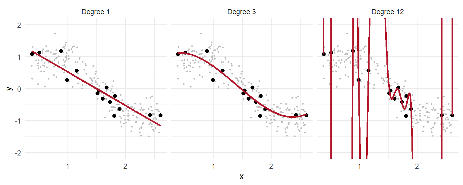

Figure 11.1: Three models fitted to the same 15 training points (black). The straight line is too simple, the degree-3 curve follows the pattern, and the degree-12 curve passes close to every training point but wanders far from the new points (grey).

The straight line is too simple to follow the wave: it underfits. The degree-3 curve captures the pattern. The degree-12 curve bends to pass close to every training point, and in doing so follows the noise, swinging far away from where new points actually lie. Measured on the training points, it would look like the best model; measured on new points, it is the worst. The prediction error of every degree from 1 to 12 shows the general pattern:

rmse <- function(observed, predicted) sqrt(mean((observed - predicted)^2))

errors <- bind_rows(lapply(1:12, function(d) {
  fit <- lm(y ~ poly(x, d), data = train_points)
  tibble(degree = d,
         training = rmse(train_points$y, predict(fit, train_points)),
         new_data = rmse(new_points$y, predict(fit, new_points)))
}))

errors |>
  tidyr::pivot_longer(-degree, names_to = "data", values_to = "error") |>
  ggplot(aes(x = degree, y = error, colour = data)) +
  geom_line(linewidth = 1) +
  geom_point() +
  scale_x_continuous(breaks = 1:12) +
  scale_colour_manual(values = c(training = "grey50", new_data = "#b2182b"),
                      labels = c(training = "Training points", new_data = "New points")) +
  scale_y_log10() +
  labs(x = "Flexibility (polynomial degree)", y = "Prediction error (RMSE, log scale)",
       colour = NULL) +
  theme_minimal(base_size = 12)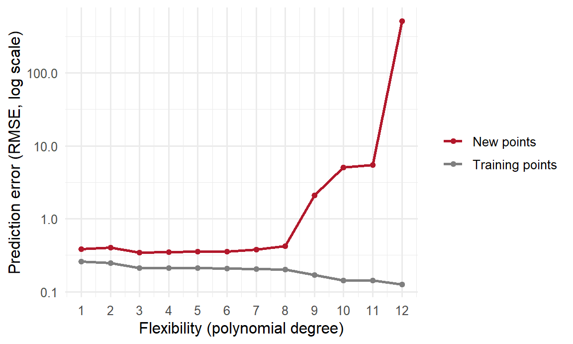

Figure 11.2: Prediction error (RMSE) on the training points and on new points, for polynomials of degree 1 to 12. Training error keeps falling as the model becomes more flexible; error on new data falls, then rises.

The training error falls steadily as the model becomes more flexible: a more flexible model can always fit its own data more closely. The error on new data falls at first, reaches its minimum at degree 3, and then rises. This U shape is known as the bias-variance trade-off. A model that is too simple has high bias: it misses part of the real pattern, whatever data it is given. A model that is too flexible has high variance: it changes a great deal from one sample to another, because it follows each sample’s noise. The best predictions come from a model in between, and the only way to find it is to measure performance on data the model did not learn from. The rest of the chapter builds that measurement into every step.

11.3 Designing a fair test

The tidymodels framework is a collection of packages that together make a fair test of a predictive model easy to carry out. Each package handles one part of the design: rsample splits the data, recipes prepares it, parsnip specifies models, workflows combines the pieces, tune tunes models, and yardstick measures performance. Loading tidymodels loads them all:

library(tidymodels)
tidymodels_prefer()

The function tidymodels_prefer() settles a few name clashes between packages in favour of tidymodels. Figure 11.3 shows how the pieces fit together: the test data is set aside before anything else happens, all choices are made with the training data alone, and the test data is used once, at the end. The rest of the chapter works through each step.

flowchart TB
  A[All data] --> B[Split:<br/>training and test]
  B --> C[Training data]
  B --> T[Test data,<br/>set aside]
  C --> D[Recipe:<br/>prepare the data]
  D --> E[Model:<br/>fit and tune with<br/>cross-validation]
  E --> F[Final model]
  T --> G[Evaluate once<br/>on the test data]
  F --> G

Figure 11.3: The machine learning workflow in tidymodels.

11.4 Data for prediction

A predictive model can only use information that would be available when the prediction is made. The university wants to act at the end of the first semester, so the model may use the students’ background, their questionnaire scores from the start of the year, and their first-semester records, but nothing from later. The questionnaire scores are calculated as before:

scores <- questionnaire |>
  mutate(
    stress_4     = 6 - stress_4,
    stress       = rowMeans(pick(stress_1:stress_6), na.rm = TRUE),
    burnout      = rowMeans(pick(burnout_1:burnout_6), na.rm = TRUE),
    support      = rowMeans(pick(support_1:support_6), na.rm = TRUE),
    satisfaction = rowMeans(pick(satisfaction_1:satisfaction_4), na.rm = TRUE)
  ) |>
  select(student_id, stress, burnout, support, satisfaction)

dropout_data <- students |>
  left_join(scores, join_by(student_id)) |>
  left_join(semesters |> filter(semester == 1) |> select(-semester), join_by(student_id)) |>
  mutate(considering_dropout = factor(considering_dropout, levels = c("Yes", "No"))) |>
  select(-student_id, -supervisor_id, -workshop, -workshop_sessions)

dim(dropout_data)

[1] 600  21

Two details matter. The outcome must be a factor, and its first level is treated as the event to predict, so the levels are set to put "Yes" first. And the workshop variables are removed: the workshop took place after the first semester, so it would not be known when the prediction is made. Using information that would not be available at the time of prediction is a form of data leakage, and it makes a model look better than it can ever be in practice.

dropout_data |> count(considering_dropout) |> mutate(share = n / sum(n))

  considering_dropout   n share
1                 Yes  90  0.15
2                  No 510  0.85

Only about 15% of students answer “Yes”. Such an imbalanced outcome is common in real prediction problems, from rare diseases to fraud, and, as the evaluation below shows, it catches out anyone who judges a model by accuracy alone.

11.5 Splitting the data

The most important rule of machine learning follows from the simulation above: never judge a model on the data it learned from. The first step is therefore to split the data. The training set is used to build and tune the model. The test set is locked away and used only once, at the very end, to estimate how the final model will perform on new students. The function initial_split() does the split, and strata makes sure that both sets have the same share of “Yes” answers:

set.seed(2026)
dropout_split <- initial_split(dropout_data, prop = 0.75, strata = considering_dropout)
dropout_train <- training(dropout_split)
dropout_test  <- testing(dropout_split)

nrow(dropout_train)

[1] 449

nrow(dropout_test)

[1] 151

Three quarters of the students are used for training and a quarter are set aside for the final test.

11.6 Preparing the data

Most models need the data prepared first: missing values filled in, categories turned into numbers, and numeric predictors put on a common scale. A recipe lists these steps:

dropout_recipe <- recipe(considering_dropout ~ ., data = dropout_train) |>
  step_impute_median(all_numeric_predictors()) |>
  step_dummy(all_nominal_predictors()) |>
  step_normalize(all_numeric_predictors())

The first line says that considering_dropout is the outcome and every other column (.) is a predictor. The step step_impute_median() then replaces each missing numeric value with the median of that variable. The step step_dummy() turns each categorical predictor into dummy variables: 0/1 columns, one per category except a reference category, as lm() did automatically in Chapter 8. Finally, step_normalize() turns every numeric predictor into z-scores, so they are on the same scale; some models, such as k-nearest neighbours below, depend on distances and need this.

The recipe only describes the steps. To see what it produces, prep() estimates what it needs from the training data (the medians, the means and standard deviations), and bake() applies it:

dropout_recipe |>
  prep() |>
  bake(new_data = NULL) |>
  glimpse()

Rows: 449
Columns: 25
$ age                      <dbl> 0.24508282, -0.38372967, 0.87389531, 1.293103…
$ financial_worry          <dbl> -0.7012103, -0.7012103, -0.7012103, 1.9008013…
$ stress                   <dbl> -0.07328352, 0.78371678, 1.95645404, -0.29880…
$ burnout                  <dbl> -0.5660882, 0.1216109, 2.1847084, 1.0385432, …
$ support                  <dbl> -1.48927219, -1.70433127, 0.66131866, -0.8440…
$ satisfaction             <dbl> -1.1166487, -1.1166487, -0.4684583, -0.792553…
$ gpa                      <dbl> -0.20629899, 0.49821479, -1.55406449, -0.7576…
$ sleep_hours              <dbl> 0.705824008, -0.090694948, -1.185908512, -0.5…
$ study_hours              <dbl> -0.09621851, 0.36256496, 0.89781234, -0.78439…
$ exercise_days            <dbl> 1.5418905, -0.1263236, -0.1263236, -0.1263236…
$ caffeine_mg              <dbl> -0.41150631, 0.17158271, 1.00977318, -0.15640…
$ supervisor_meetings      <dbl> -1.50209363, -0.42757418, -0.06940103, 2.0796…
$ wellbeing                <dbl> 1.13636876, -0.04432777, -1.22502430, -0.2973…
$ considering_dropout      <fct> No, No, No, No, No, No, No, No, No, No, No, N…
$ gender_Male              <dbl> -0.9489638, -0.9489638, -0.9489638, 1.0514340…
$ faculty_Health.Sciences  <dbl> 1.6539530, -0.6032655, 1.6539530, -0.6032655,…
$ faculty_Humanities       <dbl> -0.4072635, -0.4072635, -0.4072635, 2.4499443…
$ faculty_Natural.Sciences <dbl> -0.4365273, -0.4365273, -0.4365273, -0.436527…
$ faculty_Social.Sciences  <dbl> -0.4861964, -0.4861964, -0.4861964, -0.486196…
$ programme_PhD            <dbl> -0.6445746, 1.5479556, -0.6445746, 1.5479556,…
$ study_mode_Part.time     <dbl> -0.6342138, -0.6342138, 1.5732436, -0.6342138…
$ employment_None          <dbl> 0.9966636, -1.0011130, -1.0011130, -1.0011130…
$ employment_Part.time.job <dbl> -0.7039606, 1.4173703, -0.7039606, 1.4173703,…
$ has_children_Yes         <dbl> -0.5449999, -0.5449999, -0.5449999, -0.544999…
$ lives_away_Yes           <dbl> 1.1662426, 1.1662426, -0.8555448, 1.1662426, …

In this code, new_data = NULL means “the training data the recipe was prepared on”. In the result, gender has become gender_Male, faculty has become four dummy columns, and all the numbers are now z-scores.

ImportantNo peeking at the test data

The medians, means, and standard deviations are estimated from the training data only, and then applied unchanged to the test data. If they were calculated from all the data, information from the test set would leak into the model, and the test would no longer be a fair one. Recipes and workflows handle this automatically, which is one of the best reasons to use them.

11.7 Specifying and fitting a model

The parsnip package specifies models in one consistent way, whatever package does the actual work. Here is logistic regression:

logistic_spec <- logistic_reg()
logistic_spec

Logistic Regression Model Specification (classification)

Computational engine: glm 

A workflow combines the recipe and the model, so they always travel together:

logistic_wf <- workflow() |>
  add_recipe(dropout_recipe) |>
  add_model(logistic_spec)

logistic_fit <- fit(logistic_wf, data = dropout_train)

The function fit() prepares the recipe on the training data and fits the model to the prepared data, in one step.

11.8 Evaluating a classifier

The model is now judged on the test students. The function augment() adds the model’s predictions to the test data: the predicted class (.pred_class) and the predicted probability of each class (.pred_Yes, .pred_No):

test_results <- augment(logistic_fit, new_data = dropout_test)
test_results |>
  select(considering_dropout, .pred_class, .pred_Yes) |>
  head()

# A tibble: 6 × 3
  considering_dropout .pred_class .pred_Yes
  <fct>               <fct>           <dbl>
1 No                  No            0.216  
2 No                  No            0.0279 
3 No                  No            0.00744
4 Yes                 No            0.424  
5 No                  No            0.0114 
6 No                  No            0.0298 

The simplest measure is accuracy: the share of students classified correctly. The yardstick package calculates it:

test_results |> accuracy(truth = considering_dropout, estimate = .pred_class)

# A tibble: 1 × 3
  .metric  .estimator .estimate
  <chr>    <chr>          <dbl>
1 accuracy binary         0.834

An accuracy of 83% sounds good. But a “model” that ignores every predictor and says “No” for every student would be right 85% of the time, because most students answer “No”, while finding not one of the students at risk. For an imbalanced outcome, accuracy is a misleading measure.

A better measure is the ROC AUC (the area under the ROC curve). It is the probability that, of one student who considered dropping out and one who did not, the model gives the first a higher predicted probability than the second. An AUC of 0.5 is no better than a coin toss, and 1.0 is perfect. Unlike accuracy, it is not fooled by an imbalanced outcome. It uses the predicted probabilities:

test_results |> roc_auc(truth = considering_dropout, .pred_Yes)

# A tibble: 1 × 3
  .metric .estimator .estimate
  <chr>   <chr>          <dbl>
1 roc_auc binary         0.840

An AUC of 0.84 means the model ranks an at-risk student above a not-at-risk student about 84% of the time: a useful model. Chapter 12 looks at classification measures in much more detail, including how to choose the threshold at which a student is flagged.

11.9 Overfitting in practice

The simulation at the start of the chapter showed overfitting with a flexible curve. The same happens with real data. A dramatic example is k-nearest neighbours (k-NN) with \(k = 1\). It predicts each student’s outcome by finding the single most similar student in the training data and copying their answer. On the training data, every student’s nearest neighbour is themselves, so it can never be wrong:

knn1_wf <- workflow() |>
  add_recipe(dropout_recipe) |>
  add_model(nearest_neighbor(neighbors = 1) |> set_mode("classification"))
knn1_fit <- fit(knn1_wf, data = dropout_train)

augment(knn1_fit, new_data = dropout_train) |> roc_auc(considering_dropout, .pred_Yes)

# A tibble: 1 × 3
  .metric .estimator .estimate
  <chr>   <chr>          <dbl>
1 roc_auc binary             1

augment(knn1_fit, new_data = dropout_test) |> roc_auc(considering_dropout, .pred_Yes)

# A tibble: 1 × 3
  .metric .estimator .estimate
  <chr>   <chr>          <dbl>
1 roc_auc binary         0.671

The model scores perfectly on the training data, and much more poorly on new students. The training score was an illusion: the model had memorised the training students, not learned anything that carries over. It is the degree-12 curve again, and the reason every model in this book is tested on data it has not seen.

11.10 Cross-validation

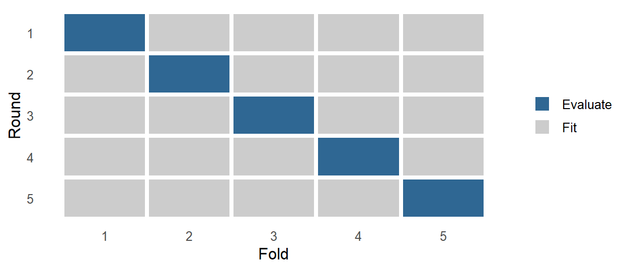
The test set is used only once, at the end. During model building, however, models and settings often need to be compared, and neither the training data (that would reward overfitting) nor the test set (that would use it up) can be used to judge them. Cross-validation solves this by reusing the training data. The training data is split into, say, 10 equal parts, called folds. The model is fitted on 9 folds and its performance measured on the fold left out; this is repeated 10 times, leaving out each fold in turn, and the 10 performance measures are averaged. Every student is used for evaluation exactly once, always by a model that did not see them during fitting. Figure 11.4 shows the idea with 5 folds.

Figure 11.4: Five-fold cross-validation: in each round, the model is fitted on four folds (grey) and evaluated on the fifth (dark).

The function vfold_cv() creates the folds, and fit_resamples() fits and evaluates the workflow on each:

set.seed(2026)
dropout_folds <- vfold_cv(dropout_train, v = 10, strata = considering_dropout)

logistic_cv <- fit_resamples(logistic_wf, resamples = dropout_folds,
                             metrics = metric_set(roc_auc, accuracy))
collect_metrics(logistic_cv)

# A tibble: 2 × 6
  .metric  .estimator  mean     n std_err .config        
  <chr>    <chr>      <dbl> <int>   <dbl> <chr>          
1 accuracy binary     0.862    10 0.00806 pre0_mod0_post0
2 roc_auc  binary     0.804    10 0.0303  pre0_mod0_post0

The cross-validated AUC, about 0.8, is an honest estimate of how the model will perform on new students, obtained without touching the test set. The standard error (std_err) shows how much the estimate varies across folds.

11.11 Tuning a model

Many models have settings that are not learned from the data but must be chosen beforehand, such as \(k\) in k-nearest neighbours or the degree of the polynomials in the simulation. They are called hyperparameters, to distinguish them from the parameters, such as regression coefficients, that the model learns. The best value is found by tuning: trying several values and comparing them with cross-validation.

A decision tree (explained fully in Chapter 12) predicts by asking a series of yes-or-no questions, such as whether stress is above 3.5. Its depth, the number of questions in a row, is a hyperparameter that controls its flexibility. A shallow tree is too simple to capture the patterns and underfits; a very deep tree can fit the training data closely, noise included, and overfits. In the model specification, tune() marks the hyperparameter to be tuned:

tree_spec <- decision_tree(tree_depth = tune(), min_n = 10, cost_complexity = 0) |>
  set_mode("classification")

tree_wf <- workflow() |>
  add_recipe(dropout_recipe) |>
  add_model(tree_spec)

The function tune_grid() tries each value in a grid, using the same cross-validation folds:

set.seed(2026)
tree_tuning <- tune_grid(tree_wf, resamples = dropout_folds,
                         grid = tibble(tree_depth = 1:10),
                         metrics = metric_set(roc_auc))

autoplot(tree_tuning) + theme_minimal(base_size = 12)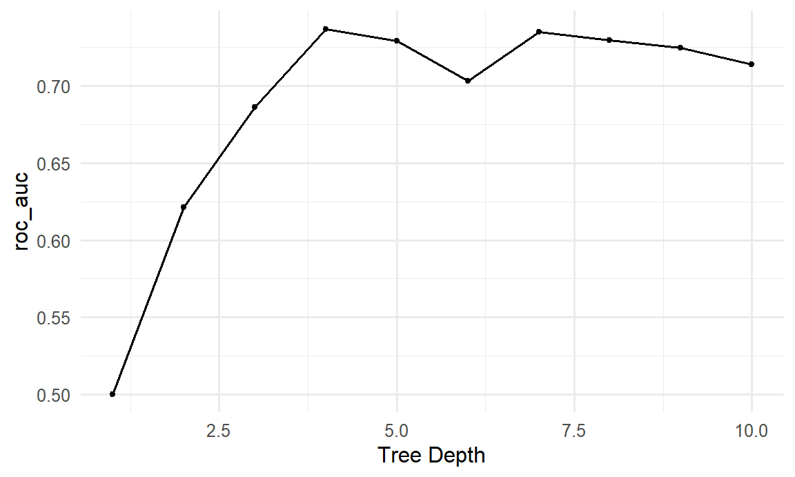

Figure 11.5: Cross-validated ROC AUC of decision trees of different depths.

The pattern is the new-data curve of Figure 11.2 seen from the other side: a tree of depth 1 is no better than chance, the AUC rises as the tree grows, and beyond a moderate depth it levels off and dips slightly as the deeper trees start to overfit. The function select_best() picks the best depth, here 4:

best_depth <- select_best(tree_tuning, metric = "roc_auc")
best_depth

# A tibble: 1 × 2
  tree_depth .config         
       <int> <chr>           
1          4 pre0_mod04_post0

11.12 The final test

Only now, with the model chosen, is the test set used. The function finalize_workflow() plugs the best depth into the workflow, and last_fit() fits it on the whole training set and evaluates it once on the test set:

final_tree <- tree_wf |>
  finalize_workflow(best_depth) |>
  last_fit(dropout_split, metrics = metric_set(roc_auc, accuracy))
collect_metrics(final_tree)

# A tibble: 2 × 4
  .metric  .estimator .estimate .config        
  <chr>    <chr>          <dbl> <chr>          
1 accuracy binary         0.828 pre0_mod0_post0
2 roc_auc  binary         0.815 pre0_mod0_post0

The same is done for logistic regression, for comparison:

final_logistic <- last_fit(logistic_wf, dropout_split, metrics = metric_set(roc_auc, accuracy))
collect_metrics(final_logistic)

# A tibble: 2 × 4
  .metric  .estimator .estimate .config        
  <chr>    <chr>          <dbl> <chr>          
1 accuracy binary         0.834 pre0_mod0_post0
2 roc_auc  binary         0.840 pre0_mod0_post0

The tuned tree reaches an AUC of 0.81; plain logistic regression, 0.84. The more flexible model is not the better one. In this data, the risk of dropout rises steadily with stress and falls steadily with support, so a simple smooth model captures the pattern well, while a tree, which splits the data into boxes, captures it less well. Trying a simple model first, and making a complex one earn its place, is one of the most useful habits in machine learning.

WarningPredictions about people

A model that flags students “at risk” affects real people. Before such a model is used, the consequences of its errors must be considered: a student flagged by mistake may be treated differently, and a student who is missed receives no help. The model should be checked separately for different groups, such as women and men or part-time and full-time students, because a model with a good AUC overall can still be unfair to a particular group. And its purpose matters: in this study, the right use is to offer support earlier, never to penalise.

NoteIn your field: business and finance

Banks use exactly these methods to predict which loan applicants will repay. The credit_data dataset from the modeldata package (installed with tidymodels) records real loan applications, with whether each loan turned out well or badly. The same workflow applies:

data(credit_data, package = "modeldata")

set.seed(1)
credit_split <- initial_split(credit_data, strata = Status)

credit_wf <- workflow() |>
  add_recipe(
    recipe(Status ~ ., data = training(credit_split)) |>
      step_impute_median(all_numeric_predictors()) |>
      step_impute_mode(all_nominal_predictors()) |>
      step_dummy(all_nominal_predictors())
  ) |>
  add_model(logistic_reg())

last_fit(credit_wf, credit_split) |> collect_metrics()

# A tibble: 3 × 4
  .metric     .estimator .estimate .config        
  <chr>       <chr>          <dbl> <chr>          
1 accuracy    binary         0.782 pre0_mod0_post0
2 roc_auc     binary         0.824 pre0_mod0_post0
3 brier_class binary         0.148 pre0_mod0_post0

The step step_impute_mode() fills missing categories with the most common one. Only the data and the outcome have changed; every step is the same. The output also shows the Brier score, brier_class, another measure of how good the predicted probabilities are: 0 is perfect, and lower is better.

11.13 Common misconceptions

Predictive modelling has its own characteristic mistakes, most of them versions of testing a model on what it already knows.

• “A model that fits the training data well will predict well.” Training performance rewards overfitting; only performance on new data counts.
• “A more complex model is a better model.” Beyond a point, flexibility adds variance, not accuracy. Simple models often predict as well.
• “High accuracy means a good classifier.” For an imbalanced outcome, a model that predicts the common class every time can have high accuracy and no value.
• “The test set can be used to choose between models.” Every use of the test set for a decision makes it less of a test. Choices are made with cross-validation; the test set is used once.
• “A good predictor is a cause.” Prediction needs association, not causation; a predictive model says nothing about what would happen if a predictor were changed.

11.14 Chapter review

11.14.1 Summary

• Supervised learning predicts an outcome (classification for categories, regression for numbers); unsupervised learning finds structure. Prediction is a different research aim from explanation, judged by performance on new data.
• A model generalises when it learns the pattern and not the noise. Training error keeps falling as models become more flexible, while error on new data falls and then rises: the bias-variance trade-off.
• tidymodels designs a fair test: it splits data (rsample), prepares it (recipes), specifies models (parsnip), combines them (workflows), tunes them (tune), and measures performance (yardstick).
• Split the data into training and test sets, stratified by the outcome, and use the test set only once, at the end. Use only information available at the time of prediction.
• A recipe prepares data (imputation, dummy variables, normalisation) using the training data only, so no information leaks from the test set.
• Accuracy misleads for imbalanced outcomes; the ROC AUC is a better summary.
• Cross-validation estimates performance honestly without using the test set. Hyperparameters are chosen by tuning with cross-validation. Simple models often predict as well as complex ones; try them first.
• Predictions about people raise questions of fairness and use.

11.14.2 Key terms

Machine learning, supervised learning, unsupervised learning, classification, regression, prediction, explanation, generalisation, overfitting, underfitting, bias-variance trade-off, imbalanced outcome, training set, test set, stratified split, recipe, imputation, dummy variable, normalisation, data leakage, model specification, workflow, accuracy, ROC AUC, k-nearest neighbours, cross-validation, fold, hyperparameter, parameter, tuning, decision tree.

11.15 Exercises

The playground has these and more, with hints and solutions.

1. Remove the questionnaire scores (stress, burnout, support, satisfaction) from dropout_data and fit the logistic regression workflow again. Report how much the cross-validated AUC falls, and what that says about the questionnaire.
2. Split the data 80/20 instead of 75/25 with a different seed, and describe how much the test AUC of the logistic model changes, and why it might.
3. Tune k-nearest neighbours over neighbors = c(5, 11, 21, 41) with cross-validation. Identify the best value, and compare its AUC with logistic regression.
4. Add step_zv(all_predictors()) to the recipe (it removes predictors with only one value). Look up what “zero variance” means, and explain when this step is useful.
5. In two or three sentences, explain to a university administrator why a model with 85% accuracy might still be useless for finding students at risk.
6. Repeat the polynomial simulation with 50 training points instead of 15. Describe how the error curve on new data changes, and explain why more data allows a more flexible model.

11.16 Further reading

• Tidy Modeling with R (Kuhn and Silge 2022), the book by the authors of tidymodels, is the definitive guide to the framework.
• An Introduction to Statistical Learning (James et al. 2021) explains the ideas behind overfitting, the bias-variance trade-off, cross-validation, and the methods of the next chapters.

References

James, Gareth, Daniela Witten, Trevor Hastie, and Robert Tibshirani. 2021. An Introduction to Statistical Learning: With Applications in r. 2nd ed. Springer. https://doi.org/10.1007/978-1-0716-1418-1.

Kuhn, Max, and Julia Silge. 2022. Tidy Modeling with r: A Framework for Modeling in the Tidyverse. O’Reilly Media. https://www.tmwr.org.