Introduction to Machine Learning in R
Introduction to Machine Learning in R
Judged by one thing: how well it works on new cases
Chapter 11
Polla Fattah
By the end of today you can
- tell supervised from unsupervised learning, and prediction from explanation;
- explain generalisation, overfitting, and the bias-variance trade-off;
- split data into training and test sets, and say why;
- prepare data with a recipe, and combine it with a model in a workflow;
- evaluate a classifier, and explain why accuracy can mislead;
- use cross-validation, tune hyperparameters, and run a final test.
Some questions are about what will happen
- which patients are likely to be readmitted?
- which loans are likely to fail?
- which students are likely to struggle, early enough to help?
The university wants to identify at-risk students at the end of their first semester.
Kinds of machine learning
| Kind | Data | Examples |
|---|---|---|
| supervised: classification | outcome is a category | considering dropout: yes or no |
| supervised: regression | outcome is a number | next semester’s GPA |
| unsupervised | no outcome; find structure | clustering (Chapters 9, 14) |
Many methods are familiar statistics: logistic regression is also a classifier.
Explanation and prediction
| Explanation (Chapters 7–10) | Prediction (Chapters 11–16) | |
|---|---|---|
| question | why does it happen? | what will happen for a new case? |
| judged by | sensible, well-estimated effects | accuracy on new data |
| typical models | simple, interpretable | anything that predicts well |
| main danger | confounding | overfitting |
A good predictor need not be a cause; a good explanation may predict poorly.
Generalisation
Any dataset holds two things:
- the pattern that would appear again in new data;
- the noise that belongs to this sample only.
A model that learns the pattern generalises. One that also learns the noise overfits.
Simulating overfitting
true_curve  <- function(x) sin(2 * x)
make_points <- function(n) {
  x <- runif(n, 0, 3)
  tibble(x = x, y = true_curve(x) + rnorm(n, sd = 0.3))
}
train_points <- make_points(15)
new_points   <- make_points(300)

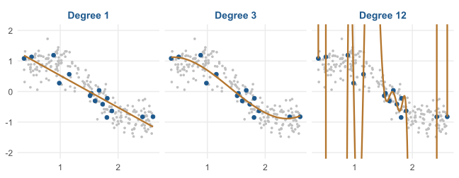
lm(y ~ poly(x, d), data = train_points)   # d = 1, 3, 12
15 noisy points from a wave, and three polynomials of increasing flexibility.
Too simple, about right, too flexible
The line underfits. Degree 3 follows the pattern. Degree 12 threads every training point and swings away from the new ones.
The bias-variance trade-off
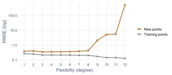
Training error keeps falling. Error on new data is lowest at degree 3, then rises.
Bias and variance
| Too simple | Too flexible |
|---|---|
| high bias | high variance |
| misses part of the real pattern | follows each sample’s noise |
| wrong whatever the data | changes greatly between samples |
The only way to find the model in between is to measure performance on data it did not learn from.
tidymodels designs a fair test
| Package | Job |
|---|---|
| rsample | split the data |
| recipes | prepare it |
| parsnip | specify models |
| workflows | combine recipe and model |
| tune | tune hyperparameters |
| yardstick | measure performance |
library(tidymodels), then tidymodels_prefer() to settle name clashes.
The workflow of a fair test
flowchart TB
  A[All data] --> B[Split]
  B --> C[Training data]
  B --> T[Test data, set aside]
  C --> D[Recipe] --> E[Fit and tune with<br>cross-validation] --> F[Final model]
  T --> G[Evaluate once]
  F --> G
All choices use the training data. The test data is used once, at the end.
Use only what is known at prediction time
dropout_data <- students |>
  left_join(scores, join_by(student_id)) |>
  left_join(semesters |> filter(semester == 1) |> select(-semester),
            join_by(student_id)) |>
  mutate(considering_dropout = factor(considering_dropout,
                                      levels = c("Yes", "No"))) |>
  select(-student_id, -supervisor_id, -workshop, -workshop_sessions)
The first factor level is the event to predict, so "Yes" comes first.
The workshop came after semester 1: using it would be data leakage.
An imbalanced outcome
Only about 15% of students answer “Yes”.
Rare outcomes are common in real prediction, from disease to fraud, and they fool anyone who judges by accuracy alone.
Never judge a model on the data it learned from
set.seed(2026)
dropout_split <- initial_split(dropout_data, prop = 0.75,
                               strata = considering_dropout)
dropout_train <- training(dropout_split)
dropout_test  <- testing(dropout_split)
449 students to train, 151 locked away for the final test.
strata keeps the same share of “Yes” in both.
A recipe prepares the data
dropout_recipe <- recipe(considering_dropout ~ ., data = dropout_train) |>
  step_impute_median(all_numeric_predictors()) |>
  step_dummy(all_nominal_predictors()) |>
step_normalize(all_numeric_predictors())| Step | Does |
|---|---|
step_impute_median() |
fills missing numbers with the median |
step_dummy() |
turns categories into 0/1 columns |
step_normalize() |
turns numbers into z-scores |
prep() and bake()
prep() estimates medians, means, and SDs from the training data; bake() applies them.
gender becomes gender_Male; faculty becomes four dummy columns.
No peeking at the test data
The medians, means, and SDs come from the training data only.
They are applied unchanged to the test data.
Calculated from all the data, they would leak test information into the model. Recipes and workflows prevent this automatically.
Model and workflow
logistic_spec <- logistic_reg()

logistic_wf <- workflow() |>
  add_recipe(dropout_recipe) |>
  add_model(logistic_spec)

logistic_fit <- fit(logistic_wf, data = dropout_train)
parsnip specifies models the same way whatever package does the work.
A workflow keeps recipe and model together; fit() prepares and fits in one step.
Predictions on the test students
test_results <- augment(logistic_fit, new_data = dropout_test)
test_results |> accuracy(truth = considering_dropout, estimate = .pred_class)
augment() adds .pred_class and the probabilities .pred_Yes, .pred_No.
Accuracy: 83%. It sounds good.
Accuracy misleads for rare outcomes
| “Model” | Accuracy | At-risk students found |
|---|---|---|
| logistic regression | 83% | some |
| always say “No” | 85% | none |
A “model” that ignores every predictor scores as well or better, and helps no one.
ROC AUC
The probability that, of one student who considered dropping out and one who did not, the model ranks the first higher.
| AUC | 0.5 | 1.0 | this model |
|---|---|---|---|
| meaning | coin toss | perfect | 0.84 |
Not fooled by imbalance. Chapter 12 goes further, including thresholds.
Overfitting in real data: 1-nearest neighbour
knn1_wf <- workflow() |>
  add_recipe(dropout_recipe) |>
add_model(nearest_neighbor(neighbors = 1) |> set_mode("classification"))| Data | AUC |
|---|---|
| training | 1.00 |
| test | 0.67 |
On training data each student’s nearest neighbour is themselves. The model memorised; it did not learn.
Comparing models without the test set
Models and settings need comparing during building.
- the training data would reward overfitting;
- the test set would be used up.
Cross-validation reuses the training data.
Cross-validation
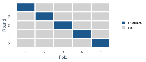
Fit on four folds, evaluate on the fifth, rotate, average. Every student is evaluated once, by a model that never saw them.
Cross-validation in tidymodels
set.seed(2026)
dropout_folds <- vfold_cv(dropout_train, v = 10, strata = considering_dropout)

logistic_cv <- fit_resamples(logistic_wf, resamples = dropout_folds,
                             metrics = metric_set(roc_auc, accuracy))
collect_metrics(logistic_cv)
Cross-validated AUC ≈ 0.80 (standard error 0.030): an honest estimate, without touching the test set.
Parameters and hyperparameters
| Learned from data? | Example | |
|---|---|---|
| parameter | yes | regression coefficients |
| hyperparameter | no, chosen beforehand | k in k-NN, tree depth, polynomial degree |
Tuning tries several hyperparameter values and compares them with cross-validation.
Tuning a decision tree’s depth
tree_spec <- decision_tree(tree_depth = tune(), min_n = 10,
                           cost_complexity = 0) |>
  set_mode("classification")

tree_tuning <- tune_grid(tree_wf, resamples = dropout_folds,
                         grid = tibble(tree_depth = 1:10),
                         metrics = metric_set(roc_auc))
A tree asks yes-or-no questions in a row. Its depth controls flexibility. tune() marks what to tune.
Depth against AUC
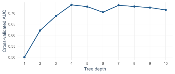
Depth 1 is chance; AUC rises, then levels off and dips as deep trees overfit. select_best() picks depth 4.
The final test
final_tree <- tree_wf |>
  finalize_workflow(best_depth) |>
  last_fit(dropout_split, metrics = metric_set(roc_auc, accuracy))

final_logistic <- last_fit(logistic_wf, dropout_split,
                           metrics = metric_set(roc_auc, accuracy))
last_fit() fits on the whole training set and evaluates once on the test set.
The simple model wins
| Model | Test AUC |
|---|---|
| tuned decision tree | 0.81 |
| logistic regression | 0.84 |
Dropout risk rises steadily with stress and falls with support: a smooth model captures that; a tree cuts it into boxes.
Try a simple model first, and make a complex one earn its place.
Predictions about people
- a student flagged by mistake may be treated differently;
- a student who is missed receives no help;
- a good overall AUC can hide unfairness to one group;
- the right use here is to offer support earlier, never to penalise.
Check the model separately for women and men, part-time and full-time students.
In your field: business and finance
credit_wf <- workflow() |>
  add_recipe(recipe(Status ~ ., data = training(credit_split)) |>
               step_impute_median(all_numeric_predictors()) |>
               step_impute_mode(all_nominal_predictors()) |>
               step_dummy(all_nominal_predictors())) |>
  add_model(logistic_reg())
last_fit(credit_wf, credit_split) |> collect_metrics()
Loan applications and whether they turned out well. Only the data changed.
The Brier score measures probability quality: 0 is perfect.
Practical lab: the Chapter 11 playground
Work through the playground exercises in your browser, with hints and solutions.
The browser version uses base R for AUC and cross-validation; the download uses tidymodels.
Practical exercises 1–3: data and models
- Remove the questionnaire scores: how much does the AUC fall?
- Split 80/20 with another seed: how much does the test AUC move?
- Tune k-NN over 5, 11, 21, 41 neighbours and compare with logistic regression.
Practical exercises 4–6: judgement
- What does
step_zv()do, and when is it useful? - Explain to an administrator why 85% accuracy may be useless.
- With 50 training points, how does the new-data error curve change?
Try this yourself
Think of a prediction your own field needs.
- what outcome, and when must the prediction be made?
- which variables would be known at that moment?
- how rare is the outcome, and which measure would you use?
- what would the cost of each kind of error be?
Troubleshooting guide (Part 1)
| Symptom | Likely cause |
|---|---|
| a near-perfect training score | overfitting; judge on new data |
| a model better than seems possible | data leakage from the future |
| high accuracy, no cases found | an imbalanced outcome |
| the event level is predicted backwards | the outcome factor’s first level is not the event |
Troubleshooting guide (Part 2)
| Symptom | Likely cause |
|---|---|
| test set used to pick the model | it is no longer a test; use cross-validation |
| preprocessing on all the data | test information leaked; use a recipe |
| unequal “Yes” shares in train and test | split not stratified |
| a complex model loses to a simple one | the pattern is smooth; that is fine |
Completion checklist
Misconceptions to leave behind (Part 1)
| Misconception | Better mental model |
|---|---|
| a good training fit predicts well | only new-data performance counts |
| more complex is better | flexibility adds variance |
| high accuracy means a good classifier | not for imbalanced outcomes |
Misconceptions to leave behind (Part 2)
| Misconception | Better mental model |
|---|---|
| the test set can choose between models | choose by cross-validation; test once |
| a good predictor is a cause | prediction needs association only |
The chapter in one sentence
A predictive model is only as good as its performance on data it has never seen, so design the test before you build the model.
Next: Chapter 12
The next chapter compares classifiers:
- decision trees and random forests;
- k-nearest neighbours and support vector machines;
- comparing models fairly;
- the confusion matrix and choosing a threshold;
- imbalanced outcomes and fairness.
Questions
If a model flagged students at risk, who should see the flag?
What would you do for a student it missed?