Research data often contains many possible predictors for rather few cases. A questionnaire with dozens of items, several rounds of measurement, and a background survey can easily supply 50 predictors for a sample of 60 or 100 people. Ordinary regression estimates a coefficient for every predictor, and with that much freedom it can fit its own data almost perfectly while predicting new cases badly: the overfitting of Chapter 11, now in its most common form. The problem is made worse when predictors are correlated, as questionnaire items usually are.
This chapter introduces two families of methods that make many predictors usable. Regularised regression (ridge, lasso, and elastic net) keeps the familiar linear model but shrinks its coefficients towards zero, trading a little fit on the training data for much better predictions. Boosting builds a flexible model from many small decision trees, each correcting the errors of the ones before. The chapter also introduces the measures used to judge numeric predictions. The outcome is now a number, so this is a regression problem in the machine learning sense of Chapter 11. In the study, it answers the tenth research question (RQ10): the university’s academic advisers meet every student at the end of the first year, and would like to know from year-one information which students are heading for a low final GPA, so that extra support can be planned.
TipBy the end of this chapter you will be able to
Measure the accuracy of numeric predictions with RMSE, MAE, and R², and compare them with a baseline.
Explain why ordinary regression overfits when there are many predictors.
Fit and tune ridge, lasso, and elastic net regression, and read which predictors the lasso keeps.
Explain how boosting builds a model from many small trees, and tune an XGBoost model.
Choose between models with cross-validation, and report the final model’s accuracy on the test set.
The advisers meet students at the end of year one, so the model may use only what is known by then: the students’ background, their questionnaire answers, and their records from semesters 1 and 2. The outcome is GPA in semester 4.
This time, every questionnaire item is used as a separate predictor, rather than the four scale scores, to show how the methods cope with many related predictors. The semester records are in long format (one row per student per semester); for prediction, they are needed in wide format, one row per student, with a column for each measure in each semester. pivot_wider() from Chapter 3 does this:
The argument names_glue builds the new column names, such as gpa_s1 and sleep_hours_s2, and inner_join() keeps only students who have a final GPA. That is an important limitation: the 37 students who left the programme have no final GPA, so the model can only predict the final GPA of students who stay. (Chapter 6 showed that the leavers were not a random group, so the model should not be used to judge them.)
The split, folds, and recipe follow Chapter 11. With a numeric outcome, strata splits the outcome into quartiles and samples within each, so that both sets cover the full range of GPAs. The recipe adds step_impute_mode() to fill in any missing categories:
Each error (or residual) is the actual value minus the prediction, and three measures summarise them. The MAE (mean absolute error) is the average size of the errors, ignoring their sign; here, (0.2 + 0.1 + 0.3 + 0.1 + 0.4) / 5 = 0.22 GPA points. The RMSE (root mean squared error) squares the errors, averages them, and takes the square root. Squaring gives large errors more weight, so the RMSE is always at least as large as the MAE, and much larger when there are a few big misses. R², in yardstick, is the squared correlation between the predictions and the actual values: as in Chapter 8, the share of the variation in the outcome that the predictions capture, from 0 to 1. The yardstick package calculates all three:
# A tibble: 3 × 3
  .metric .estimator .estimate
  <chr>   <chr>          <dbl>
1 rmse    standard       0.249
2 mae     standard       0.220
3 rsq     standard       0.785
MAE and RMSE are in the units of the outcome, here GPA points, which makes them easy to explain: “the model’s predictions are typically off by about 0.2 GPA points”. Lower is better. R² has no units; higher is better.
A number on its own means little, so every model should be compared with a baseline: the simplest possible prediction. For a numeric outcome, the baseline predicts the same value, the training mean, for everyone, which is what parsnip’s null_model() does:
# A tibble: 2 × 6
  .metric .estimator  mean     n std_err .config
  <chr>   <chr>      <dbl> <int>   <dbl> <chr>
1 mae     standard   0.256    10 0.00738 pre0_mod0_post0
2 rmse    standard   0.323    10 0.0104  pre0_mod0_post0
Predicting the average GPA for everyone gives an RMSE of 0.32. Any useful model must do clearly better. (The R² of the baseline cannot be calculated, because its predictions do not vary, so it is left out here.)
13.3 Ordinary regression with many predictors
The obvious model is the multiple regression of Chapter 8, using every predictor:
# A tibble: 3 × 6
  .metric .estimator  mean     n std_err .config
  <chr>   <chr>      <dbl> <int>   <dbl> <chr>
1 mae     standard   0.172    10 0.00615 pre0_mod0_post0
2 rmse    standard   0.218    10 0.0105  pre0_mod0_post0
3 rsq     standard   0.564    10 0.0420  pre0_mod0_post0
A cross-validated RMSE of 0.218, much better than the baseline. With 422 training students and 51 predictors, ordinary regression works reasonably well. But watch what happens with fewer students. Many theses have samples of 50 or 60, so here is the same model fitted to 60 randomly chosen training students, and tested on the test set:
# A tibble: 3 × 3
  .metric .estimator .estimate
  <chr>   <chr>          <dbl>
1 rmse    standard      0.526
2 mae     standard      0.430
3 rsq     standard      0.0456
On its own 60 students, the model looks excellent: an RMSE of 0.11. On new students, its RMSE is 0.53, worse than predicting the average GPA for everyone. With 51 coefficients estimated from 60 students, the model has enough freedom to fit the noise in its sample, and the coefficients that fit the noise do not carry over. In the extreme, with as many predictors as students, a regression can fit its data perfectly and predict nothing.
The problem is made worse by multicollinearity: many of the predictors are strongly correlated (six stress items, two semesters of GPA), and regression struggles to divide the credit between correlated predictors. Their coefficients become large, unstable, and sometimes of opposite signs, cancelling each other out on the training data but not on new data.
13.4 Regularised regression
Regularisation tackles this directly: it fits the regression while penalising large coefficients. Ordinary regression chooses the coefficients that minimise the sum of squared errors. Regularised regression minimises
\[
\text{sum of squared errors} + \lambda \times \text{size of the coefficients}.
\]
The penalty\(\lambda\) (lambda) sets how much large coefficients cost. With \(\lambda = 0\), this is ordinary regression; as \(\lambda\) grows, the coefficients are pulled, or shrunk, towards zero. A little shrinkage costs almost nothing in fit to the training data, but makes the model much more stable on new data. Because the penalty depends on the size of the coefficients, the predictors must be on the same scale, which the recipe’s step_normalize() ensures. There are three versions, which differ in how “size” is measured. Ridge regression uses the sum of the squared coefficients: it shrinks all coefficients towards zero and shares the credit among correlated predictors, but keeps every predictor in the model. The lasso (least absolute shrinkage and selection operator) uses the sum of the absolute coefficients (Tibshirani 1996). It shrinks too, but it also sets some coefficients to exactly zero, removing those predictors, so it also selects predictors and leaves a simpler model. The elastic net mixes the two, with a mixture parameter that runs from 0 (pure ridge) to 1 (pure lasso).
In tidymodels, all three are linear_reg() with the glmnet engine, with penalty for \(\lambda\) and mixture for the mix. The 60 students are now refitted with a lasso:
# A tibble: 3 × 3
  .metric .estimator .estimate
  <chr>   <chr>          <dbl>
1 rmse    standard       0.204
2 mae     standard       0.168
3 rsq     standard       0.616
From the same 60 students, the lasso’s RMSE on new students is 0.20, against 0.53 for ordinary regression. The penalty kept the model from chasing noise.
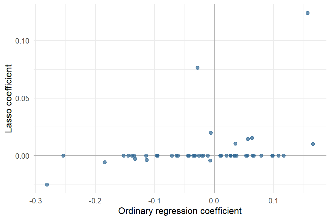
The difference lies in the coefficients. Figure 13.1 compares, predictor by predictor, the coefficients that ordinary regression and the lasso estimated from the same 60 students:
Figure 13.1: Coefficients estimated from the same 60 students by ordinary regression (horizontal axis) and by the lasso (vertical axis), one point per predictor. Ordinary regression spreads large coefficients over many predictors; the lasso sets most of them to zero and keeps a few, smaller ones.
Ordinary regression gives every predictor a coefficient, many of them large and in both directions: with 60 students, it cannot tell real effects from the chance patterns of this sample, so it fits both. Some of its coefficients make no sense. Semester 1 GPA, one of the best predictors of final GPA, receives a negative coefficient (-0.03), and caffeine in semester 2 receives a larger one (0.17) than semester 2 GPA (0.16). The lasso gives both GPA measures positive coefficients (0.08 and 0.12) and almost nothing to caffeine. The lasso keeps only 12 of the 51 predictors and shrinks even those. This is the sense in which shrinkage trades fit for stability: coefficients pulled towards zero cannot chase the noise of one sample, so they carry over better to the next.
13.4.1 Choosing the penalty
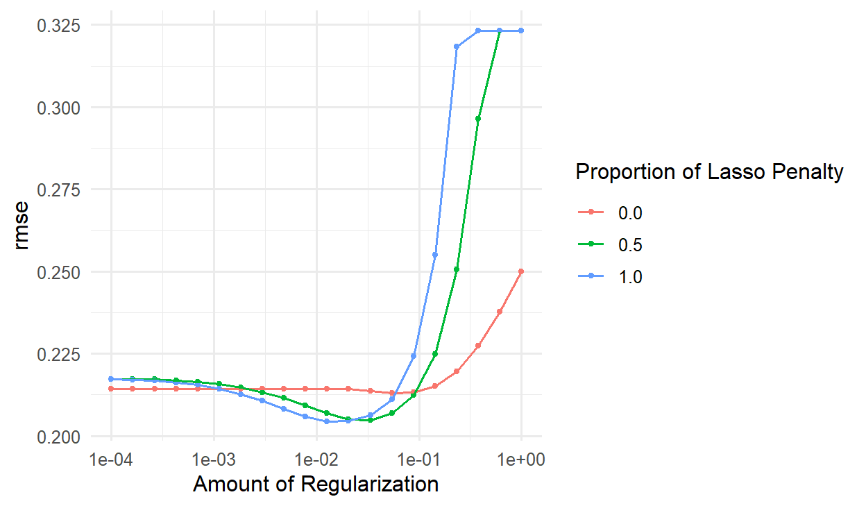
The penalty and mixture are hyperparameters, so they are tuned with cross-validation, now on the full training set. The grid tries 20 penalties, spread evenly on a logarithmic scale from 0.0001 to 1, for ridge, an even elastic net, and lasso:
Figure 13.2: Cross-validated RMSE of ridge (mixture 0), elastic net (0.5), and lasso (1) regression for a range of penalties.
Figure 13.2 shows the typical pattern. With a tiny penalty, all three behave like ordinary regression. As the penalty grows, the RMSE improves, reaches a minimum, and then rises steeply once the penalty is so large that it shrinks away real effects too. At the far right, the lasso has shrunk every coefficient to zero and predicts the mean for everyone: its RMSE equals the baseline’s.
show_best(glmnet_tuning, metric ="rmse", n =3)
# A tibble: 3 × 8
  penalty mixture .metric .estimator  mean     n std_err .config
    <dbl>   <dbl> <chr>   <chr>      <dbl> <int>   <dbl> <chr>
1  0.0127     1   rmse    standard   0.204    10 0.00871 pre0_mod33_post0
2  0.0207     1   rmse    standard   0.205    10 0.00811 pre0_mod36_post0
3  0.0336     0.5 rmse    standard   0.205    10 0.00813 pre0_mod38_post0
The best combination is a mixture of 1 with a penalty of 0.013, but the top few are nearly identical. The function select_best() picks the winner, and finalize_workflow() plugs it in:
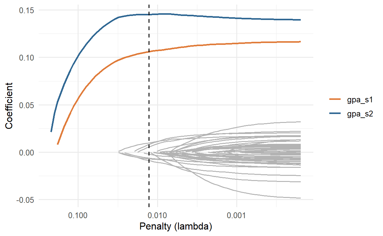
Of 51 predictors, the lasso keeps 10. Because the predictors are normalised, the coefficients are comparable: the change in predicted final GPA for a one-standard-deviation difference in the predictor. Year-one GPA dominates. A student whose semester 2 GPA is one standard deviation above average is predicted to finish about 0.15 GPA points higher; the other predictors add small adjustments.
Figure 13.3 shows how the lasso arrives at this. As the penalty decreases from left to right, predictors enter the model one by one, and the two GPA measures enter first.
Figure 13.3: Lasso coefficient paths. Each line is one predictor’s coefficient as the penalty decreases from left to right. The dashed line marks the chosen penalty.
WarningSelected is not the same as causal
It is tempting to read the lasso’s choice as a list of what matters for grades. It is not. Sleep affects GPA in the wellbeing data (Chapter 8), yet the lasso drops the sleep variables, because their effect is already reflected in year-one GPA: once the model knows a student’s past grades, knowing their sleep adds little to the prediction. Among correlated predictors, the lasso tends to keep one and drop the others, and which one it keeps can change from sample to sample. Use the lasso to predict, and use the methods of Chapters 8 and 10 to explain.
13.5 Boosting
The second family builds a model in a completely different way. Boosting starts with a very simple prediction, the average, and then adds small decision trees one at a time, each fitted to the errors of the model so far. The first tree learns the biggest pattern in the errors; the next tree learns what the first missed; and so on. Each tree’s contribution is scaled down by a learning rate (for example 0.1), so the model improves in small steps and no single tree dominates. Hundreds of trees, each weak on its own, add up to a strong model.
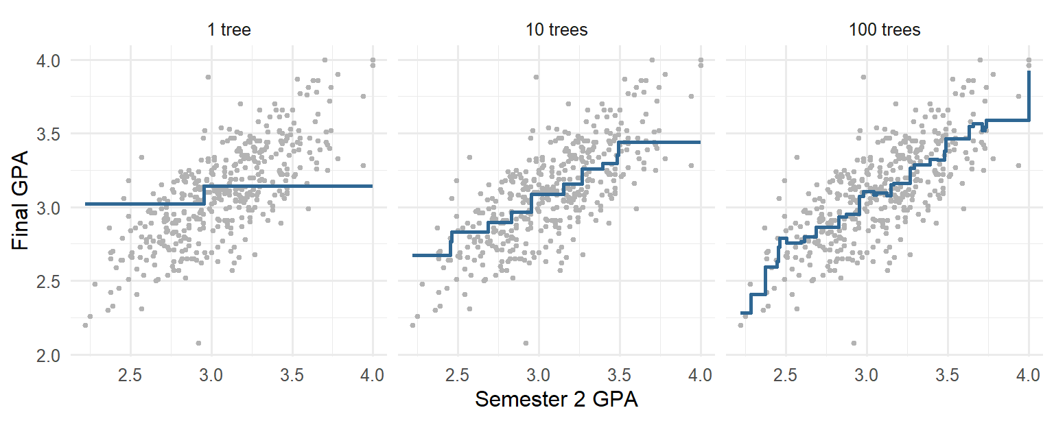
Figure 13.4 shows the idea with a single predictor, semester 2 GPA, and trees with a single split. After one tree, the prediction is a single step; after ten, a staircase; after a hundred, a curve that follows the data.
Figure 13.4: Boosting with one predictor. Predicted final GPA from semester 2 GPA after 1, 10, and 100 trees, each with a single split.
Boosting is closely related to the random forests of Chapter 12, which also combine many trees. The difference is that a forest grows its trees independently and averages them, while boosting grows them in sequence, each correcting the last. XGBoost (“extreme gradient boosting”) is a fast, popular implementation (Chen and Guestrin 2016), and one of the most successful methods for tables of data. Its main hyperparameters are the number of trees, the learning rate, and the depth of each tree. A small learning rate needs more trees; deeper trees capture interactions between predictors. Here, 500 trees are used, and the learning rate and depth are tuned:
# A tibble: 3 × 8
  tree_depth learn_rate .metric .estimator  mean     n std_err .config
       <dbl>      <dbl> <chr>   <chr>      <dbl> <int>   <dbl> <chr>
1          1       0.03 rmse    standard   0.212    10 0.00968 pre0_mod2_post0
2          2       0.01 rmse    standard   0.213    10 0.00928 pre0_mod4_post0
3          1       0.01 rmse    standard   0.213    10 0.00834 pre0_mod1_post0
The best settings use trees of depth 1, and the best RMSE is 0.212. Trees of depth 1 use one predictor each, so a boosted model built from them adds up separate effects of each predictor, with no interactions. That the shallowest trees work best is another sign that the wellbeing data has no strong interactions for the trees to find.
13.6 Comparing the models
All the models were evaluated with the same folds, so their cross-validated RMSEs can be compared directly:
# A tibble: 6 × 3
  model              rmse std_err
  <chr>             <dbl>   <dbl>
1 Lasso             0.204 0.00871
2 Elastic net       0.205 0.00813
3 XGBoost           0.212 0.00968
4 Ridge             0.213 0.00938
5 Linear regression 0.218 0.0105
6 Baseline (mean)   0.323 0.0104
The function filter_parameters() keeps only the tuning results with a given mixture, so the best ridge, elastic net, and lasso can be picked out separately.
The regularised models come out on top, followed closely by XGBoost, and all of them improve on ordinary regression. The differences between the best models are smaller than their standard errors. The lasso is chosen: it predicts as well as any, and it uses only 10 predictors, which makes it the easiest to explain and to use.
13.7 The final test
As always, the test set is used once, at the end. The function last_fit() fits the chosen model on the full training set and evaluates it on the test students:
# A tibble: 3 × 4
  .metric .estimator .estimate .config
  <chr>   <chr>          <dbl> <chr>
1 rmse    standard       0.192 pre0_mod0_post0
2 mae     standard       0.161 pre0_mod0_post0
3 rsq     standard       0.648 pre0_mod0_post0
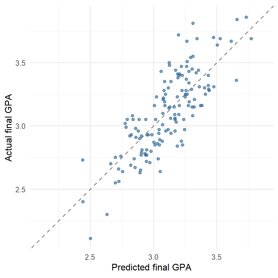
On new students, the lasso’s predictions are off by 0.16 GPA points on average (MAE), with an RMSE of 0.19, and they capture 65% of the variation in final GPA. Figure 13.5 compares the predictions with the actual final GPAs.
collect_predictions(final_lasso) |>ggplot(aes(x = .pred, y = final_gpa)) +geom_abline(linetype ="dashed", colour ="grey50") +geom_point(alpha =0.6, colour ="#2f6793") +coord_obs_pred() +labs(x ="Predicted final GPA", y ="Actual final GPA") +theme_minimal(base_size =12)
Figure 13.5: Predicted and actual final GPA for the test students. Points on the dashed line are predicted perfectly.
The function coord_obs_pred() from tune gives both axes the same range, so the diagonal is at 45 degrees. The predictions are less spread out than the actual values: the model predicts the most extreme students closer to the average than they turn out to be. This is normal for any model that cannot predict perfectly, and it means that the model is most reliable for students in the middle of the range.
A last comparison shows how much all the year-one measures add to past grades. A plain regression on the two year-one GPAs alone gives:
# A tibble: 3 × 4
  .metric .estimator .estimate .config
  <chr>   <chr>          <dbl> <chr>
1 rmse    standard       0.193 pre0_mod0_post0
2 mae     standard       0.163 pre0_mod0_post0
3 rsq     standard       0.641 pre0_mod0_post0
Its test RMSE, 0.193, is practically the same as the lasso’s 0.192. For the advisers, this is a useful, if humbling, result: past grades are by far the best predictor of future grades, and the questionnaire and semester records add little on top. That does not make sleep, stress, or support irrelevant to grades (Chapter 8 showed that they matter), but their influence is already visible in the year-one grades.
NoteIn your field: engineering
Engineers predict the strength of concrete from its recipe. The concrete data in the modeldata package records the compressive strength of 1030 concrete samples, with the amounts of cement, water, and six other ingredients, and the age of the sample in days (Yeh 1998). Strength rises with age, but less and less, and the ingredients interact: exactly the kind of structure where boosting shines.
# A tibble: 2 × 4
  .metric .estimator .estimate .config
  <chr>   <chr>          <dbl> <chr>
1 rmse    standard      10.6   pre0_mod0_post0
2 rsq     standard       0.603 pre0_mod0_post0
collect_metrics(xgb_concrete_fit)
# A tibble: 2 × 4
  .metric .estimator .estimate .config
  <chr>   <chr>          <dbl> <chr>
1 rmse    standard       4.54  pre0_mod0_post0
2 rsq     standard       0.926 pre0_mod0_post0
As the code shows, workflow() also accepts a formula in place of a recipe. Boosting cuts the RMSE from 10.6 to 4.5 megapascals. The lesson of this chapter and the last is the same from both sides: flexible models win when the data has curves and interactions, and simple models are just as good when it does not. Only a fair comparison can tell which case you are in.
13.8 Common misconceptions
Predictive regression invites a few characteristic misreadings.
“More predictors always help.” Each extra coefficient is another chance to fit noise; with few cases, adding predictors can make predictions worse.
“The predictors the lasso keeps are the ones that matter.” The lasso keeps the predictors that help prediction, and among correlated predictors it keeps one more or less arbitrarily.
“A low RMSE means every prediction is accurate.” The RMSE is a typical error; predictions for students at the extremes are pulled towards the average and can be far off.
“Boosting is always better than regression.” Boosting wins when the data has curves and interactions; on smooth data, regularised regression predicts as well and is easier to explain.
13.9 Chapter review
13.9.1 Summary
For numeric predictions, the MAE and RMSE measure the typical error in the units of the outcome (lower is better), and R² the share of variation captured. Always compare with a baseline that predicts the mean.
With many predictors relative to the number of cases, and correlated predictors, ordinary regression overfits: excellent on the training data, poor on new data.
Regularised regression penalises large coefficients. Ridge shrinks all coefficients; the lasso also sets some to zero, selecting predictors; the elastic net mixes the two. The penalty and mixture are tuned by cross-validation, and the predictors must be normalised.
The predictors a lasso selects are useful for prediction, not evidence of causes.
Boosting adds small trees one at a time, each fitted to the errors of the model so far. XGBoost’s main hyperparameters are the number of trees, the learning rate, and the tree depth.
On the wellbeing data, regularised regression and boosting predict final GPA about equally well, and year-one GPA carries most of the information. On data with curves and interactions, boosting can be far better.
The playground has these and more, with hints and solutions.
Calculate the MAE and RMSE of the tiny example by hand (or with basic R arithmetic), and check them against yardstick. Change one prediction so that it is off by 1.0 GPA point, and explain which measure changes more, and why.
Repeat the 60-student experiment with 150 students, and report the gap between ordinary regression and the lasso.
Fit a ridge regression (mixture 0) with the best ridge penalty, compare its coefficients with the lasso’s, and count how many are exactly zero.
Replace the 22 questionnaire items with the four scale scores (as in Chapter 11), and describe how the cross-validated RMSE of the lasso changes.
Tune XGBoost with trees = c(100, 500, 1000) and a learning rate of 0.03, and describe what happens to the RMSE as trees are added.
Write two sentences for the academic advisers explaining what an RMSE of 0.2 means for an individual student’s predicted GPA.
13.11 Further reading
Tidy Modeling with R(Kuhn and Silge 2022) covers regularised regression and boosted trees in tidymodels, including more efficient tuning methods.
An Introduction to Statistical Learning(James et al. 2021) explains ridge regression, the lasso, and boosting clearly, with the ideas behind why shrinkage helps.
Tibshirani’s paper introducing the lasso (Tibshirani 1996) is a classic of modern statistics.
References
Chen, Tianqi, and Carlos Guestrin. 2016. “XGBoost: A Scalable Tree Boosting System.”Proceedings of the 22nd ACM SIGKDD International Conference on Knowledge Discovery and Data Mining, 785–94. https://doi.org/10.1145/2939672.2939785.
James, Gareth, Daniela Witten, Trevor Hastie, and Robert Tibshirani. 2021. An Introduction to Statistical Learning: With Applications in r. 2nd ed. Springer. https://doi.org/10.1007/978-1-0716-1418-1.
Kuhn, Max, and Julia Silge. 2022. Tidy Modeling with r: A Framework for Modeling in the Tidyverse. O’Reilly Media. https://www.tmwr.org.
Tibshirani, Robert. 1996. “Regression Shrinkage and Selection via the Lasso.”Journal of the Royal Statistical Society: Series B (Methodological) 58 (1): 267–88. https://doi.org/10.1111/j.2517-6161.1996.tb02080.x.
Yeh, I-Cheng. 1998. “Modeling of Strength of High-Performance Concrete Using Artificial Neural Networks.”Cement and Concrete Research 28 (12): 1797–808. https://doi.org/10.1016/S0008-8846(98)00165-3.