Many of the things researchers most want to study cannot be measured directly. Stress, burnout, satisfaction, intelligence, motivation, and quality of life are constructs (Chapter 5): ideas that exist only through their effects on what people say and do. A questionnaire approaches such a construct indirectly, through several items that are each expected to reflect it, and the researcher then has to show that the items really do measure what they are meant to. At the same time, a dataset with many variables often contains patterns that no single variable reveals, such as groups of people with a similar profile across all of them.
Multivariate methods analyse many variables at once, and this chapter introduces three of them. Principal component analysis summarises many variables with a few. Factor analysis checks whether questionnaire items measure the underlying traits they are meant to, and Cronbach’s alpha checks whether they do so consistently. Cluster analysis sorts people into groups with similar profiles. In the study, they answer two research questions: whether the 22 questionnaire items measure stress, burnout, supervisor support, and satisfaction as intended (RQ6), a question every examiner of a questionnaire study will ask, and whether there are distinct profiles of students (RQ7).
TipBy the end of this chapter you will be able to
Explain why a construct is measured with several items, and what a latent variable is.
Explore the correlations among many variables at once.
Run a principal component analysis, and decide how many components to keep.
Explain the difference between principal component analysis and factor analysis.
Run an exploratory factor analysis, and interpret factor loadings, cross-loadings, and reversed items.
Check the reliability of a questionnaire scale with Cronbach’s alpha.
Group cases with k-means and hierarchical clustering, choose the number of clusters, and describe the clusters as summaries rather than natural groups.
A single questionnaire item is a poor measure of a construct. The answer to “I feel unable to control important things in my studies” depends on the student’s stress, but also on how they read the question that day, on their mood, and on how they use the answer scale. Each item therefore carries two things: a signal from the construct, and noise of its own. A latent variable is the construct thought to lie behind the items: it is not observed, but it is assumed to cause part of every answer.
Averaging several items keeps the signal, which all items share, and lets the noise, which differs from item to item, partly cancel out. A simulation shows how much this helps. It creates a “true” stress level for 600 imaginary students, then six items, each equal to the true level plus its own random noise, and compares how closely one item and the average of several items follow the true level:
In this simulation, one item correlates only about 0.68 with the true stress level, while the average of six items correlates about 0.92. This is why questionnaires use several items for each construct, and why the items are combined into a scale score (Chapter 3).
The approach rests on an assumption that must be checked: that the items of a scale really reflect one common construct, and not several. If some stress items actually measured tiredness, averaging them would mix two things. Chapter 5 called this construct validity. The methods in this chapter provide evidence for it: factor analysis shows whether the items group as intended, and Cronbach’s alpha shows whether the items of each group agree with each other, which Chapter 5 called internal consistency.
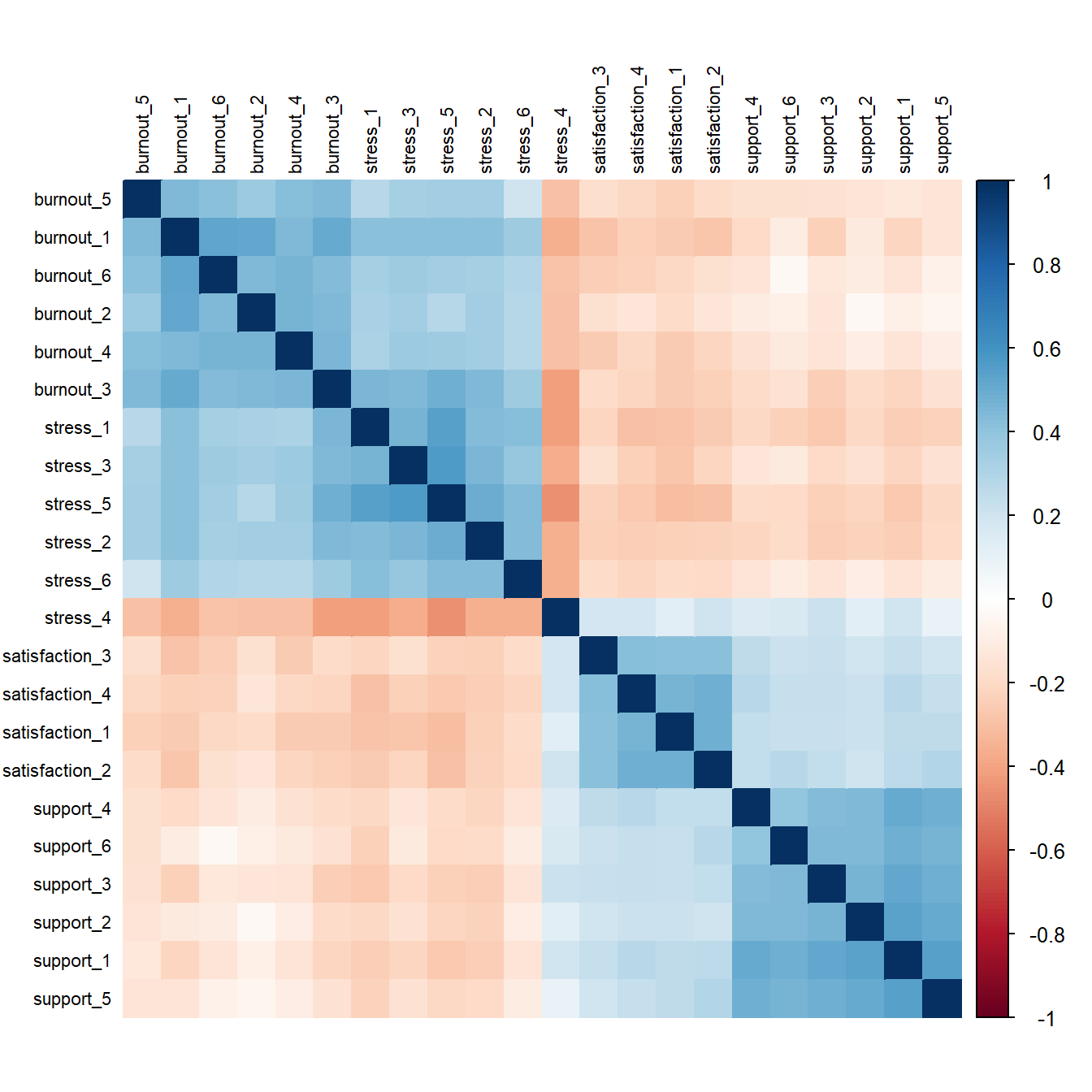
With 22 items, there are 231 correlations between pairs of items, far too many to read one by one. A picture helps. The corrplot package draws a correlation matrix as a grid of coloured squares, and order = "hclust" sorts the items so that those that correlate strongly sit together:
library(corrplot)corrplot(cor(items, use ="pairwise.complete.obs"),method ="color", order ="hclust", tl.col ="black", tl.cex =0.7)
Figure 9.1: Correlations among the 22 questionnaire items, sorted so that similar items are next to each other.
Blocks of related items stand out along the diagonal, one for each scale, just as the idea of latent variables predicts: items that share a construct correlate with each other. Blue squares show positive correlations and red negative. The stress and burnout blocks also correlate with each other, and one item, stress_4, is red against the other stress items, because it is worded the other way round. The methods in this chapter turn this picture into numbers.
9.3 Principal component analysis
Principal component analysis (PCA) replaces many correlated variables with a few new ones, called principal components, that together keep most of the information. The first component is the combination of the variables that captures as much of their variation as possible. The second captures as much as possible of what is left, and so on.
Two items that correlate strongly, such as “I feel emotionally drained by my studies” and “I feel exhausted when I think about my thesis”, illustrate the idea. Most students who score high on one score high on the other, so one combined score, their average for example, keeps most of what the two items tell. PCA does this for all the variables at once, and finds the best combinations automatically.
9.3.1 Running PCA
The function prcomp() runs PCA, and scale. = TRUE puts every variable on the same scale first, which is almost always wanted. PCA needs complete data, so na.omit() keeps only the students who answered every item:
Only 396 of the 600 students answered all 22 items: a small share of missing answers per item adds up to many incomplete students. Factor analysis, below, can use the incomplete students too.
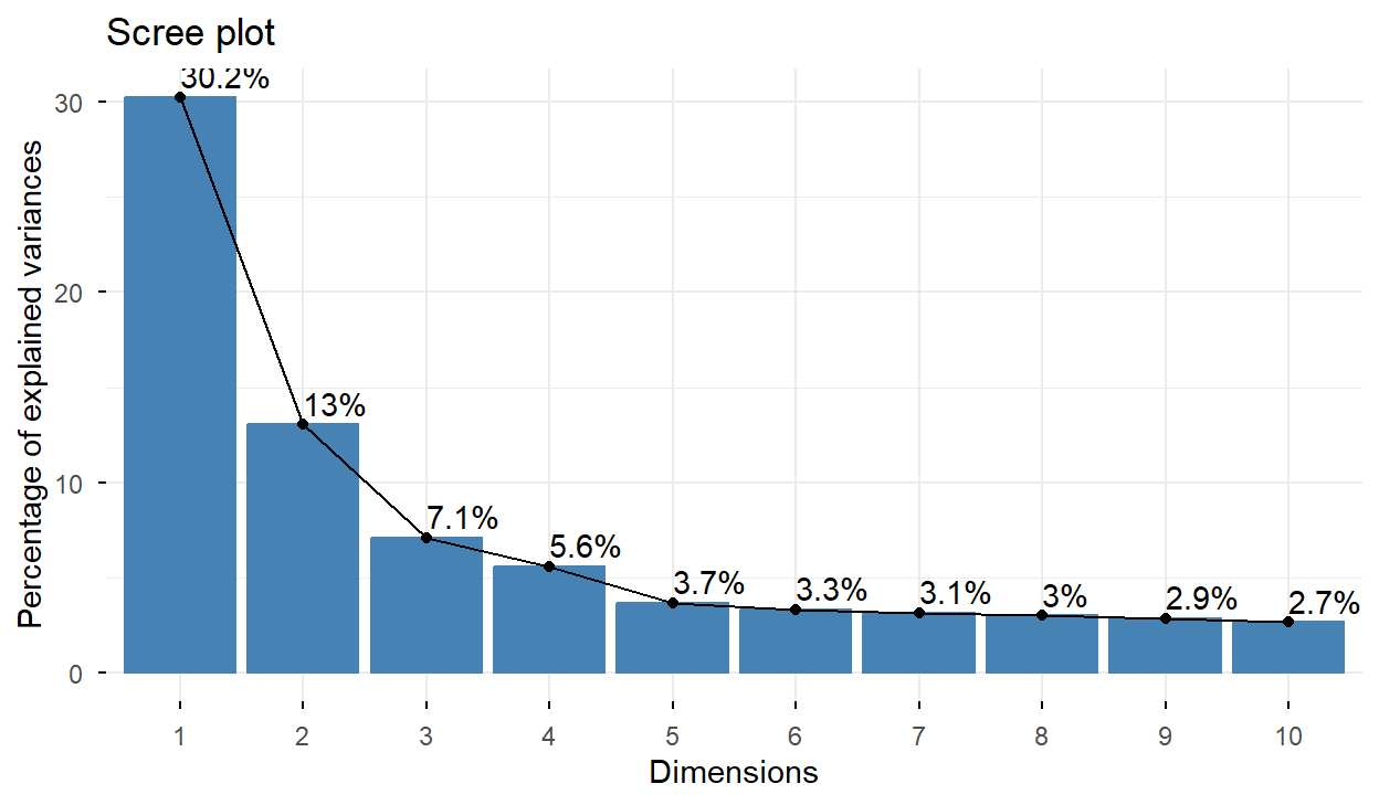
The table shows how much of the total variation each component captures. The first component alone captures 30%, and the first four together 56%.
9.3.2 The number of components
No single rule decides how many components to keep, so researchers use several. The Kaiser rule keeps components whose eigenvalue, the amount of variation they capture, is greater than 1, that is, more than one original variable’s worth; here, 4 components pass. The scree plot shows the eigenvalues in order, and the researcher looks for the “elbow” where the line flattens out. Parallel analysis compares the eigenvalues with those from random data of the same size, and keeps the components that beat random data; it is the most reliable of the three.
The factoextra package draws a scree plot directly:
Figure 9.2: Scree plot: the share of variation captured by each principal component.
The line drops steeply for four components and flattens after that. Parallel analysis, from the psych package, agrees:
library(psych)set.seed(1)parallel <-fa.parallel(items, fa ="fa", plot =FALSE)
Parallel analysis suggests that the number of factors = 4 and the number of components = NA
parallel$nfact
[1] 4
All three methods point to four dimensions, matching the four scales the questionnaire was designed to measure.
9.3.3 PCA and factor analysis compared
PCA and factor analysis are often confused, and many theses use one when they mean the other. The difference lies in what they assume. PCA simply summarises the variables: the components are combinations of the items, with no claim about why the items are related, and it is used to reduce many variables to a few, for example before a further analysis. Factor analysis assumes the model of the first section: that each item is caused by one or more latent variables, called factors, plus error of its own. A student answers the stress items the way they do because they are stressed. Factor analysis is therefore the method for checking whether a questionnaire measures the constructs it is meant to, and that is the study’s question.
9.4 Factor analysis
Exploratory factor analysis (EFA) estimates how strongly each item is related to each factor. These relationships are called loadings. Loadings run roughly from −1 to 1: close to 0 means that the item is unrelated to the factor, and a value above about 0.4 in size is usually considered a clear relationship.
The function fa() from the psych package runs the analysis. Its main arguments are the number of factors (four, from parallel analysis), the rotation, and the estimation method. Rotation turns the factors to make them easier to interpret; “oblimin” allows the factors to correlate with each other, which is realistic, since stress and burnout surely go together. The option fm = "ml" uses maximum likelihood, a common estimation method:
In the printout, cutoff = 0.3 hides small loadings so that the pattern is easy to see, and sort = TRUE groups the items by the factor they load on most. Unlike PCA, fa() uses every student, including those who skipped an item.
The table shows four clear factors. Each collects the items of one scale: the six support items on one, the stress items on another, the burnout items on a third, and the four satisfaction items on the fourth. The names ML1 to ML4 are only labels; naming the factors is the researcher’s job. The reversed item, stress_4 (“I feel confident handling problems in my studies”), loads negatively on the stress factor, which is exactly right for a reversed item: agreeing with it means less stress, and it is why the item must be reversed before the stress score is calculated (Chapter 3). One item, burnout_3 (“Deadlines make me feel overwhelmed”), loads on both the burnout and the stress factor. Reading the item, that makes sense: feeling overwhelmed by deadlines is both. Such a cross-loading item is worth discussing in a thesis, and sometimes worth rewording or removing in future studies.
Because the rotation allowed the factors to correlate, fa() also estimates how strongly they do:
The stress and burnout factors correlate strongly (about 0.66), but not so strongly that they are the same thing. The support and satisfaction factors correlate positively with each other and negatively with stress and burnout. These relationships make sense, which is itself evidence that the scales measure what they should.
9.4.1 Reliability and Cronbach’s alpha
Factor analysis shows that the items of each scale belong together. Reliability asks a related question: whether the items of a scale give consistent results (Chapter 5). The most common measure of this internal consistency is Cronbach’s alpha, which ranges from 0 to 1. It rises when the items correlate strongly with each other, and also when there are more items, for the reason shown by the simulation at the start of the chapter. As a rough guide, 0.7 or above is acceptable and 0.8 or above good for research use. The function alpha() from the psych package calculates it, after reversed items have been reversed:
All four scales are reliable, with alphas between 0.76 and 0.85. The full output of alpha() also shows what alpha would be if each item were dropped, which helps to spot a weak item.
The code writes psych::alpha() rather than alpha() because ggplot2 also has a function called alpha(), for making colours transparent. Whichever package is loaded last wins, so after loading ggplot2 (or a package that loads it, such as factoextra) a plain alpha() no longer calculates Cronbach’s alpha. The package::function() form always calls the intended function, whether or not the package is loaded.
A high alpha shows consistency, not validity. A scale can be highly reliable and still measure the wrong thing, as the target picture in Chapter 5 showed; the factor structure and the relationships with other constructs are the evidence for validity.
TipReporting the questionnaire in a thesis
A typical report: “An exploratory factor analysis (maximum likelihood, oblimin rotation) supported four factors, as indicated by parallel analysis. All items loaded on their intended factor (loadings 0.45 to 0.83 in absolute value), with one item (burnout_3) also loading on the stress factor. Internal consistency was acceptable to good (Cronbach’s α = 0.76 to 0.85).”
A further step, confirmatory factor analysis, tests whether a structure decided in advance fits the data, rather than exploring it. It is done with the lavaan package and is beyond this book.
9.5 Cluster analysis
Factor analysis groups variables. Cluster analysis groups people: it looks for groups of students whose profiles are similar to each other and different from other groups. It is a descriptive method. It does not test a hypothesis, and the groups it finds are summaries of the data, useful for describing and thinking about students, not discoveries of natural kinds of student. The study’s question about student profiles (RQ7) is accordingly exploratory (Chapter 5).
Each student is described by their average sleep, study hours, caffeine, and exercise across the semesters, and their stress, support, and satisfaction scores:
Clustering works with distances between students: how different two students’ profiles are. Caffeine is measured in hundreds of milligrams and sleep in single hours, so without adjustment caffeine would dominate every distance. The function scale() turns every variable into z-scores (Chapter 6), so each counts equally.
9.5.1 k-means clustering
k-means is the most widely used clustering method. The researcher chooses the number of clusters, \(k\), and the algorithm places \(k\) starting points at random, assigns each student to the nearest point, moves each point to the centre (the mean) of its students, and repeats the last two steps until nothing changes. Because the result depends on the random start, nstart = 25 runs the algorithm from 25 different starts and keeps the best result.
9.5.2 The number of clusters
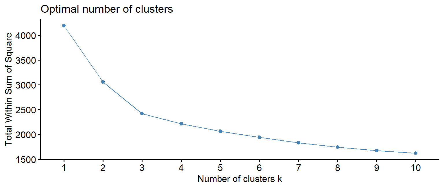
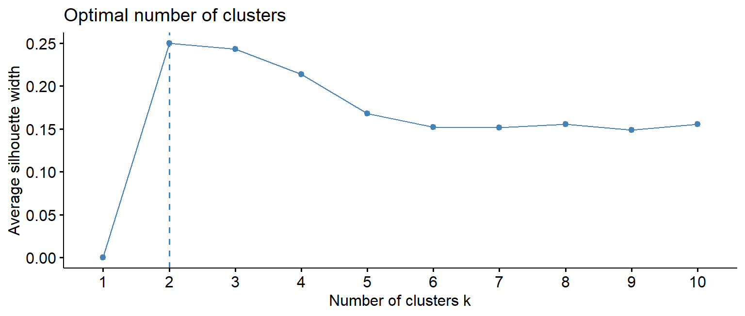
As with components, no single rule decides the number of clusters, and two guides are common. The elbow method uses the fact that the total distance of students from their cluster centres always falls as \(k\) grows, and looks for the point where adding clusters stops helping much. The silhouette measures, for each student, how much closer they are to their own cluster than to the next nearest one, from −1 to 1; a higher average silhouette means clearer clusters.
The honest conclusion is that the data does not point clearly to one number. The elbow is gentle, and the silhouette is highest for 2 clusters but only a little lower for 3 or 4. This is common with real data: groups of people overlap, and there are no sharp boundaries. The choice then rests on what is useful and interpretable, and on prior theory. The thesis, based on earlier research, expects around four student profiles, so \(k = 4\) is tried:
A cluster is only useful if its meaning can be stated. Adding the cluster to the original, unscaled data and averaging each variable by cluster shows each group’s profile:
The averages describe the groups. One is clearly balanced: the most sleep, moderate study, the most exercise, low stress, and good support. Two are overloaded: long study weeks, little sleep and exercise, high stress, and one of them (the smaller) with very high caffeine intake. The fourth combines low study hours with low support and low satisfaction: students who seem disengaged or isolated. Cluster numbers are arbitrary labels, and can change if the code is run with a different seed.
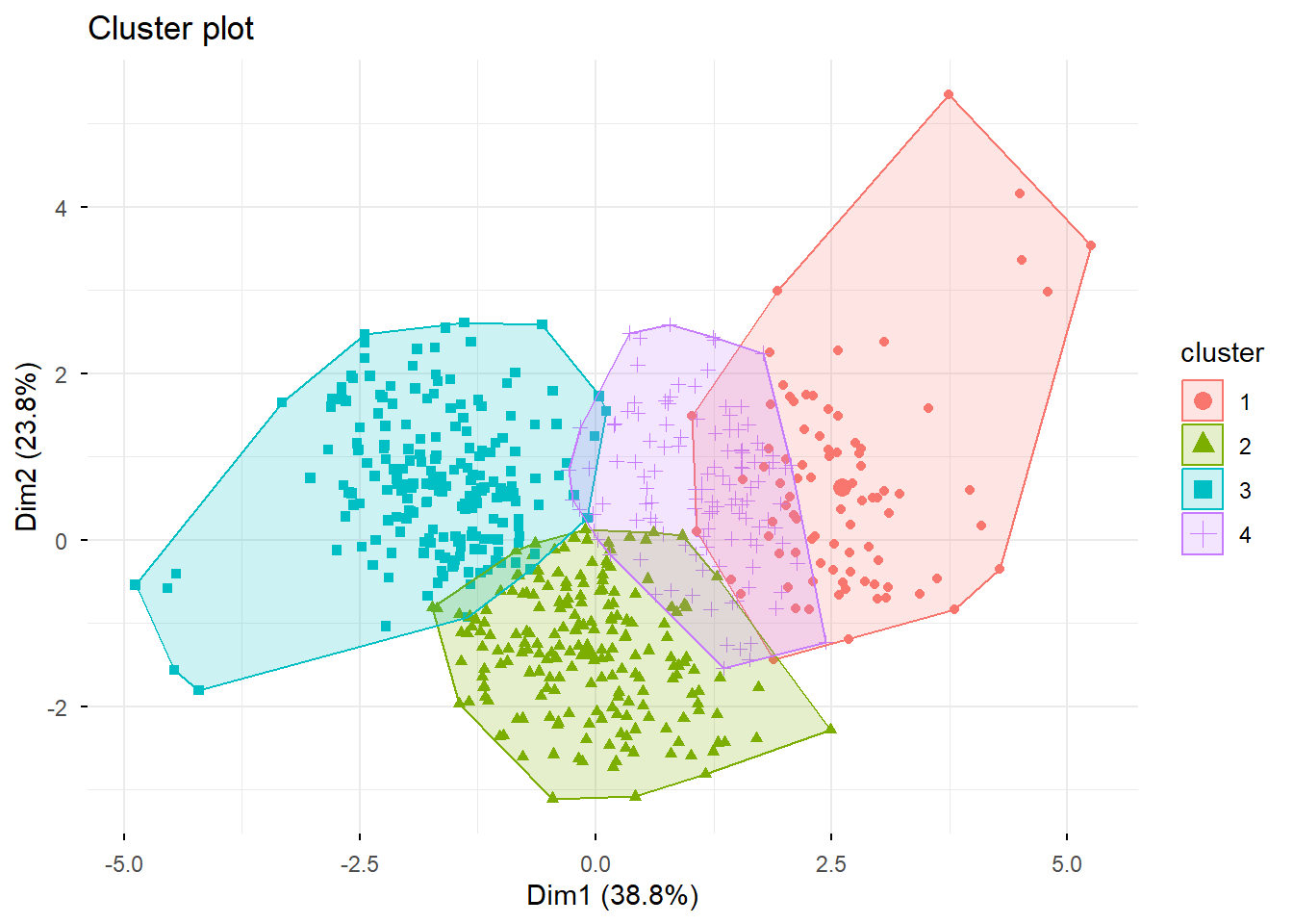
Figure 9.4 shows the clusters on the first two principal components of the profile data, a common way to see many variables in two dimensions:
fviz_cluster(clusters, data = profile_data, geom ="point", ellipse.type ="convex",ggtheme =theme_minimal())
Figure 9.4: The four k-means clusters, shown on the first two principal components of the profile data.
The clusters overlap. That is not a failure: real students do not fall into neat boxes. The profiles are useful summaries, not natural categories.
9.5.4 Hierarchical clustering
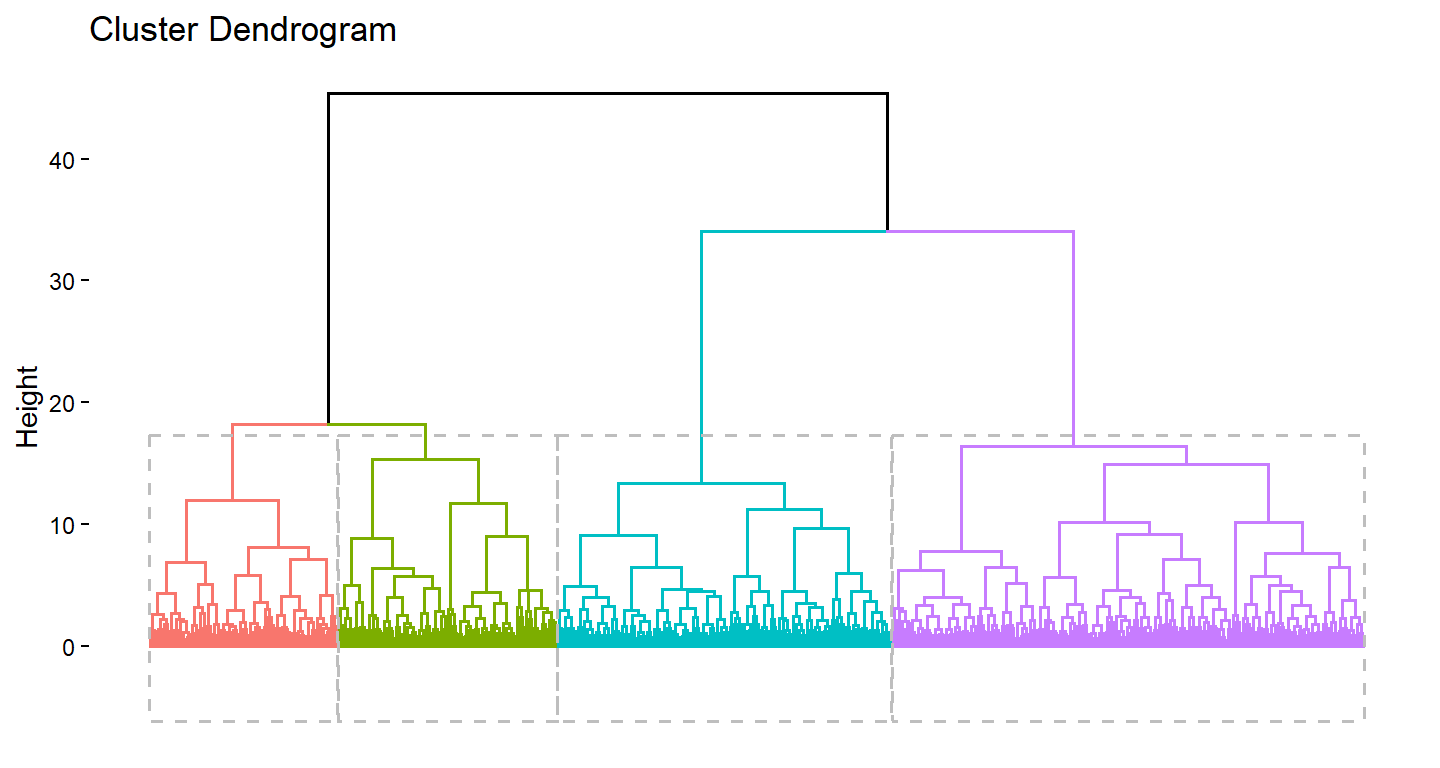
Hierarchical clustering takes a different approach. It starts with every student as their own cluster and repeatedly merges the two most similar clusters, until everyone is in one. The result is a tree, called a dendrogram, which can be cut at any height to give any number of clusters, without choosing \(k\) in advance. Ward’s method ("ward.D2") merges clusters so that they stay as compact as possible:
tree <-hclust(dist(profile_data), method ="ward.D2")fviz_dend(tree, k =4, show_labels =FALSE, rect =TRUE)
Figure 9.5: Dendrogram from hierarchical clustering (Ward’s method), cut into four clusters.
The function dist() calculates the distances between all pairs of students, and cutree() cuts the tree into groups. A cross-table shows how far the two methods agree:
hier_clusters <-cutree(tree, k =4)table(hierarchical = hier_clusters, kmeans = clusters$cluster)
They agree on the broad picture, most clearly on the balanced students, but many students switch groups between the two methods. When two reasonable methods disagree about a student, that student is near a boundary. The clearer groups, found by both methods, are the ones to trust most.
9.5.5 Clusters in random data
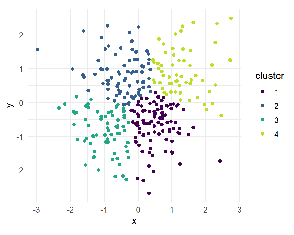
A clustering method will split any data into groups, even data that contains no groups at all. The final code makes the point with 300 points drawn entirely at random, with no structure of any kind, and asks k-means for four clusters:
Figure 9.6: k-means finds four ‘clusters’ in 300 random points that contain no groups at all.
The method obliges, and divides one round cloud into four neat regions. Nothing in its output says that the groups are artificial. The existence of clusters therefore proves nothing on its own. Before clusters are reported as meaningful, it should be checked that they make sense, that different methods broadly agree, and that the groups differ in ways that matter for the research. Chapter 14 introduces methods that allow for overlapping groups and for students who fit no group at all.
NoteIn your field: criminology and social policy
R’s USArrests dataset records rates of assault, murder, and rape per 100,000 residents, and the percentage of people living in urban areas, for the 50 US states in 1973. PCA summarises the four variables:
                        PC1  PC2
Standard deviation     1.57 0.99
Proportion of Variance 0.62 0.25
Cumulative Proportion  0.62 0.87
The first component captures about 62% of the variation: it is essentially an overall violent crime rate. The second, about 25%, mostly reflects how urban a state is. Two numbers now describe what took four.
9.6 Common misconceptions
Multivariate methods produce impressive output, which makes their limits easy to forget.
“PCA and factor analysis are the same.” PCA summarises variables; factor analysis models latent variables that cause them. Only factor analysis addresses whether a questionnaire measures its constructs.
“A high Cronbach’s alpha proves a scale is valid.” Alpha measures consistency. A scale can be consistent and still measure the wrong thing.
“Clusters are natural groups.” Clustering finds groups in any data, including random data. Clusters are summaries, and their usefulness must be argued.
“The number of factors or clusters is decided by the software.” The criteria often disagree, and the final choice is a judgement that should be justified in the thesis.
9.7 Chapter review
9.7.1 Summary
A construct is measured with several items because each item carries noise of its own; averaging keeps the shared signal. A latent variable is the unobserved construct assumed to cause the items.
A sorted correlation plot shows the structure among many variables.
PCA replaces many correlated variables with a few components that keep most of the variation. Decide how many to keep with eigenvalues above 1, the scree plot, and, most reliably, parallel analysis.
PCA summarises; factor analysis models latent variables that cause the items. Use factor analysis to check a questionnaire.
In an EFA, loadings show how strongly items relate to factors. Check that items load on their intended factor, that reversed items load negatively, and discuss cross-loadings. Oblique rotation lets factors correlate.
Cronbach’s alpha measures a scale’s internal consistency: 0.7 or above is acceptable, 0.8 or above good. Reverse reversed items first. Reliability is necessary for validity but not enough.
Cluster analysis groups people with similar profiles. Scale the variables first. k-means needs the number of clusters in advance; hierarchical clustering produces a tree that can be cut anywhere. Choose the number with the elbow and silhouette methods, theory, and interpretability.
Clustering finds groups even in random data. Clusters are useful summaries, not proof of natural groups; describe each cluster by its averages, and check that methods agree.
The playground has these and more, with hints and solutions.
Run a PCA on the six support items only. Report how much variation the first component captures, and what that suggests about the scale.
Run an EFA with three factors instead of four. Identify the scales that end up sharing a factor, and suggest why.
Calculate Cronbach’s alpha for the stress scale without reversing stress_4 first, and explain what happens.
Run k-means with 3 clusters on the profile data, describe the clusters, and identify which profiles from the 4-cluster solution were merged.
Explain, in two or three sentences for a thesis methods section, why you chose the number of clusters you did.
Change the simulation at the start of the chapter so that each item has more noise (sd = 2). Find how many items are now needed for the average to correlate at least 0.8 with the true stress level.
9.9 Further reading
An Introduction to Statistical Learning(James et al. 2021), chapter “Unsupervised Learning”, explains PCA and clustering clearly, with R examples.
James, Gareth, Daniela Witten, Trevor Hastie, and Robert Tibshirani. 2021. An Introduction to Statistical Learning: With Applications in r. 2nd ed. Springer. https://doi.org/10.1007/978-1-0716-1418-1.