Multivariate Statistical Methods
Multivariate Statistical Methods
Many variables at once: items, components, factors, and profiles
Chapter 9
Polla Fattah
By the end of today you can
- explain why a construct is measured with several items;
- explore the correlations among many variables at once;
- run a PCA and decide how many components to keep;
- tell PCA from factor analysis;
- run an exploratory factor analysis and read its loadings;
- check a scale’s reliability with Cronbach’s alpha;
- group cases with k-means and hierarchical clustering;
- describe clusters as summaries, not natural groups.
Three multivariate methods
| Method | Groups | Answers |
|---|---|---|
| principal component analysis | variables into a few summaries | how much can be kept in fewer numbers? |
| factor analysis and alpha | items into latent constructs | does the questionnaire measure what it should? (RQ6) |
| cluster analysis | people into profiles | are there distinct kinds of student? (RQ7) |
One item is a poor measure
The answer to “I feel unable to control important things in my studies” depends on:
- the student’s stress: the signal;
- how they read the question that day, their mood, how they use the scale: noise.
A latent variable is the construct thought to cause part of every answer.
Averaging keeps the signal
set.seed(42)
true_stress <- rnorm(600)
simulated_items <- sapply(1:6, function(i) true_stress + rnorm(600, sd = 1))| Items averaged | 1 | 2 | 3 | 4 | 5 | 6 |
|---|---|---|---|---|---|---|
| correlation with true stress | 0.68 | 0.81 | 0.86 | 0.89 | 0.91 | 0.92 |
The shared signal adds up; the separate noise partly cancels.
The assumption to check
Averaging works only if the items reflect one construct.
If some stress items measured tiredness, the score would mix two things.
| Evidence | Method |
|---|---|
| construct validity: items group as intended | factor analysis |
| internal consistency: items agree | Cronbach’s alpha |
22 items, 231 correlations
items <- questionnaire |> select(-student_id)
corrplot(cor(items, use = "pairwise.complete.obs"),
         method = "color", order = "hclust")
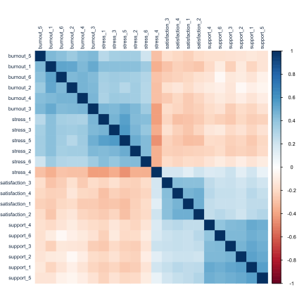
Far too many to read one by one.
order = "hclust" sorts the items so that those correlating strongly sit together.
Blocks along the diagonal
Four blocks, one per scale. stress_4 is red against the other stress items: it is worded the other way.
Principal component analysis
PCA replaces many correlated variables with a few principal components.
- the first captures as much of the variation as possible;
- the second as much as possible of what is left;
- and so on.
Two items that almost always agree can be kept as one combined score.
Running PCA
items_complete <- na.omit(items)
pca <- prcomp(items_complete, scale. = TRUE)
summary(pca)$importance[, 1:6]
scale. = TRUE puts every item on the same scale. PCA needs complete data.
Only 396 of 600 students answered all 22 items: small gaps add up.
The first component captures 30%; the first four together 56%.
How many components?
| Rule | Keeps | Here |
|---|---|---|
| Kaiser | eigenvalue > 1 | 4 components |
| scree plot | components before the elbow | 4 |
| parallel analysis | components that beat random data | 4 |
An eigenvalue is the variation a component captures. Parallel analysis is the most reliable.
The scree plot
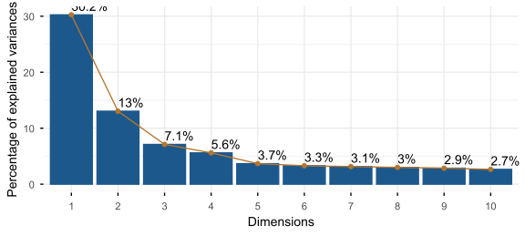
Steep for four components, flat afterwards: four dimensions, matching the four scales.
Parallel analysis
library(psych)
set.seed(1)
parallel <- fa.parallel(items, fa = "fa", plot = FALSE)
parallel$nfact
#> [1] 4
Components are kept only if they capture more than the same analysis of random data.
PCA and factor analysis are different
| PCA | Factor analysis | |
|---|---|---|
| assumes | nothing about why items relate | latent factors cause the items |
| produces | combinations of items | loadings of items on factors |
| used for | reducing many variables to few | checking a questionnaire |
Many theses use one when they mean the other.
Exploratory factor analysis
efa <- fa(items, nfactors = 4, rotate = "oblimin", fm = "ml")
print(efa$loadings, cutoff = 0.3, sort = TRUE)| Argument | Choice |
|---|---|
nfactors = 4 |
from parallel analysis |
rotate = "oblimin" |
lets factors correlate, as stress and burnout surely do |
fm = "ml" |
maximum likelihood estimation |
fa() also uses students who skipped an item.
Loadings
A loading is how strongly an item relates to a factor.
| Loading (size) | Meaning |
|---|---|
| near 0 | unrelated to the factor |
| above about 0.4 | a clear relationship |
cutoff = 0.3 hides small loadings; sort = TRUE groups items by their main factor.
Four clear factors
- the six support items on one factor;
- the stress items on another;
- the burnout items on a third;
- the four satisfaction items on the fourth.
Main loadings range from 0.45 to 0.83. The labels ML1 to ML4 are arbitrary; naming factors is the researcher’s job.
Reversed and cross-loading items
| Item | Pattern | Meaning |
|---|---|---|
stress_4 “I feel confident handling problems” |
loads negatively on stress | exactly right for a reversed item |
burnout_3 “Deadlines make me feel overwhelmed” |
loads on burnout and stress | a cross-loading, worth discussing |
A cross-loading item may be reworded or removed in future studies.
How the factors correlate
Stress and burnout correlate strongly, about 0.66, but are not the same thing.
Support and satisfaction correlate positively with each other, negatively with stress and burnout.
Relationships that make sense are themselves evidence of validity.
Cronbach’s alpha
Internal consistency: do the items of one scale give consistent results?
- rises when the items correlate strongly;
- rises when there are more items;
- 0.7 or above is acceptable, 0.8 or above good.
Reverse reversed items first.
Alpha for the four scales
q <- questionnaire
q$stress_4 <- 6 - q$stress_4
psych::alpha(q[, paste0("stress_", 1:6)])$total$raw_alpha| Scale | stress | burnout | support | satisfaction |
|---|---|---|---|---|
| alpha | 0.83 | 0.83 | 0.85 | 0.76 |
The full output shows alpha if each item were dropped, which spots a weak item.
Why psych::alpha()
ggplot2 also has an alpha(), for transparent colours.
Whichever package is loaded last wins, so a plain alpha() can call the wrong one.
package::function() always calls the intended function.
Reliability is not validity
A high alpha shows consistency.
A scale can be highly reliable and still measure the wrong thing: the target from Chapter 5.
The factor structure and relationships with other constructs are the evidence for validity.
Reporting the questionnaire
An exploratory factor analysis (maximum likelihood, oblimin rotation) supported four factors, as indicated by parallel analysis. All items loaded on their intended factor (loadings 0.45 to 0.83), with one item (burnout_3) also loading on stress. Internal consistency was acceptable to good (α = 0.76 to 0.85).
Confirmatory factor analysis, with the lavaan package, tests a structure decided in advance.
Cluster analysis groups people
Factor analysis groups variables. Cluster analysis groups people with similar profiles.
It is descriptive: it tests no hypothesis.
Its groups are summaries of the data, not discoveries of natural kinds of student. RQ7 is exploratory.
Each student’s profile
profiles <- semesters |>
  summarise(across(c(sleep_hours, study_hours, caffeine_mg, exercise_days),
                   ~ mean(.x, na.rm = TRUE)), .by = student_id) |>
  left_join(scores, join_by(student_id)) |>
  na.omit()

profile_data <- scale(profiles |> select(-student_id))
Average habits across the semesters, plus stress, support, and satisfaction.
Scale before measuring distance
Clustering works with distances between students’ profiles.
Caffeine is in hundreds of milligrams, sleep in single hours: unscaled, caffeine would dominate every distance.
scale() turns every variable into z-scores, so each counts equally.
k-means
flowchart LR
    A["Place k points<br>at random"] --> B["Assign each student<br>to the nearest"] --> C["Move each point<br>to its students' mean"]
    C -->|repeat until stable| B
The result depends on the random start, so nstart = 25 runs 25 starts and keeps the best.
Choosing the number of clusters
| Guide | Looks at |
|---|---|
| elbow method | where more clusters stop reducing within-cluster distance |
| silhouette | how much closer each student is to their own cluster than the next, −1 to 1 |
The data does not decide clearly
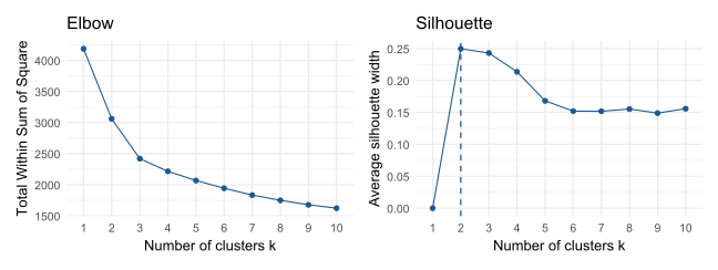
A gentle elbow; silhouette highest at 2, only a little lower at 3 or 4. Theory expects about four profiles.
Four clusters
set.seed(123)
clusters <- kmeans(profile_data, centers = 4, nstart = 25)
profiles |>
  mutate(cluster = clusters$cluster) |>
  summarise(students = n(),
            across(sleep_hours:satisfaction, ~ round(mean(.x), 1)),
            .by = cluster)
A cluster is useful only if its meaning can be stated: average each variable on the original scale.
The cluster profiles
| cluster | students | sleep | study | caffeine | exercise | stress | support | satisfaction |
|---|---|---|---|---|---|---|---|---|
| 1 | 85 | 5.1 | 41.6 | 423.7 | 1.2 | 3.6 | 2.9 | 3.0 |
| 2 | 197 | 6.7 | 18.0 | 149.8 | 2.2 | 3.4 | 2.7 | 2.5 |
| 3 | 200 | 7.2 | 23.6 | 122.9 | 3.5 | 2.6 | 3.6 | 3.8 |
| 4 | 117 | 5.8 | 40.8 | 188.1 | 1.5 | 3.6 | 3.5 | 3.3 |
Naming the profiles
| Profile | Pattern |
|---|---|
| balanced | most sleep, moderate study, most exercise, low stress, good support |
| overloaded | long study weeks, little sleep and exercise, high stress |
| overloaded, high caffeine | the same, with very high caffeine |
| disengaged or isolated | low study, low support, low satisfaction |
Cluster numbers are arbitrary and can change with the seed.
The clusters overlap
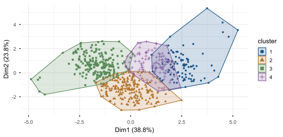
Shown on the first two principal components. Real students do not fall into neat boxes.
Hierarchical clustering
tree <- hclust(dist(profile_data), method = "ward.D2")
fviz_dend(tree, k = 4, show_labels = FALSE, rect = TRUE)
Start with every student alone, merge the two most similar clusters, repeat until one remains.
The dendrogram can be cut at any height, without choosing k in advance. Ward’s method keeps clusters compact.
Two methods, compared
They agree on the broad picture, most clearly on the balanced students.
Many students switch groups: they lie near a boundary. Trust the groups both methods find.
Clusters in random data
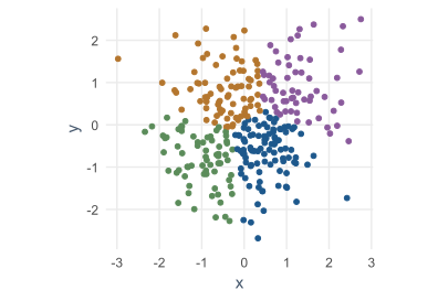
300 random points with no groups: k-means still cuts four neat wedges.
Clusters prove nothing on their own
Before reporting clusters as meaningful, check that:
- they make sense;
- different methods broadly agree;
- the groups differ in ways that matter for the research.
Chapter 14 allows overlapping groups, and students who fit no group.
In your field: criminology and social policy
Assault, murder, and rape rates, and urban population, for 50 US states.
The first component, 62%, is an overall violent crime rate; the second, 25%, how urban a state is.
Practical lab: the Chapter 9 playground
Work through the playground exercises in your browser, with hints and solutions.
Clustering and factor analysis run in the browser; every exercise also runs in RStudio.
Practical exercises 1–3: components, factors, alpha
- A PCA of the six support items: what does the first component capture?
- An EFA with three factors: which scales merge, and why?
- Alpha for stress without reversing
stress_4: what happens?
Practical exercises 4–6: clusters and noise
- k-means with 3 clusters: which profiles merged?
- Justify your number of clusters in two sentences for a thesis.
- With noisier items (
sd = 2), how many are needed for a correlation of 0.8?
Try this yourself
Take a questionnaire from your own field.
- group its items by the construct each should measure;
- list the reversed items;
- plan the EFA: number of factors, rotation, and why;
- decide what alpha you would accept, and what you would do below it.
Troubleshooting guide (Part 1)
| Symptom | Likely cause |
|---|---|
| far fewer students in PCA | na.omit() on items with scattered gaps |
| a scale’s alpha is unexpectedly low | a reversed item not recoded |
alpha() returns a colour function |
ggplot2’s alpha(); use psych::alpha() |
| an item loads on two factors | a cross-loading; read its wording |
Troubleshooting guide (Part 2)
| Symptom | Likely cause |
|---|---|
| caffeine dominates the clusters | variables not scaled |
| different clusters on every run | too few random starts; set nstart and a seed |
| the methods disagree on many students | overlapping groups; trust shared ones |
| clusters found in noise | clustering always finds groups |
Completion checklist
Misconceptions to leave behind (Part 1)
| Misconception | Better mental model |
|---|---|
| PCA and factor analysis are the same | PCA summarises; FA models latent causes |
| a high alpha proves a scale is valid | alpha measures consistency only |
Misconceptions to leave behind (Part 2)
| Misconception | Better mental model |
|---|---|
| clusters are natural groups | clustering finds groups even in random data |
| the software decides the number | criteria disagree; the choice is a justified judgement |
The chapter in one sentence
Several items measure a construct better than one; factor analysis and alpha show whether they do, and clusters summarise people without proving natural groups.
Next: Chapter 10
The next chapter models data with a structure:
- repeated measurements of the same students;
- random intercepts and random slopes;
- change in wellbeing over two years;
- students within supervisors;
- missing data and mixed models.
Questions
Which construct in your research is measured with a single item?
What would a second and third item add?