Predictive Regression
Predictive Regression
Many predictors, few cases, and a number to predict
Chapter 13
Polla Fattah
By the end of today you can
- measure numeric predictions with RMSE, MAE, and R², against a baseline;
- explain why ordinary regression overfits with many predictors;
- fit and tune ridge, lasso, and elastic net regression;
- read which predictors the lasso keeps, and what that does not mean;
- explain how boosting builds a model from small trees, and tune XGBoost;
- choose a model by cross-validation, and report the final test.
Many predictors, few cases
A questionnaire, several rounds of measurement, and a background survey can supply 50 predictors for 60 people.
Ordinary regression estimates a coefficient for each, fits its own data almost perfectly, and predicts new cases badly.
Correlated predictors, like questionnaire items, make it worse.
The question: final GPA from year one
The university’s advisers meet students at the end of year one.
| May use | May not use |
|---|---|
| background | anything after year one |
| all 22 questionnaire items | the workshop’s later effects |
| semester 1 and 2 records |
The outcome, GPA in semester 4, is a number: a regression problem.
One row per student, wide
year_one <- semesters |>
  filter(semester <= 2) |>
  pivot_wider(id_cols = student_id, names_from = semester,
              values_from = gpa:wellbeing,
              names_glue = "{.value}_s{semester}")
names_glue builds names such as gpa_s1 and sleep_hours_s2.
Only students who stayed have a final GPA
gpa_data <- students |>
  left_join(questionnaire, join_by(student_id)) |>
  left_join(year_one, join_by(student_id)) |>
  inner_join(final_gpa, join_by(student_id)) |>
  select(-student_id, -supervisor_id, -considering_dropout)
inner_join() keeps students with a final GPA: 37 who left are excluded.
The model predicts only for students who stay, and must not be used to judge the leavers.
Split, folds, and recipe
gpa_split <- initial_split(gpa_data, prop = 0.75, strata = final_gpa)
gpa_folds <- vfold_cv(gpa_train, v = 10, strata = final_gpa)

gpa_recipe <- recipe(final_gpa ~ ., data = gpa_train) |>
  step_impute_median(all_numeric_predictors()) |>
  step_impute_mode(all_nominal_predictors()) |>
  step_dummy(all_nominal_predictors()) |>
  step_normalize(all_numeric_predictors())
With a numeric outcome, strata samples within quartiles. After dummies: 51 predictors.
Errors of a numeric prediction
| Actual | Predicted | Error |
|---|---|---|
| 3.2 | 3.0 | 0.2 |
| 2.8 | 2.9 | −0.1 |
| 3.6 | 3.3 | 0.3 |
| 3.0 | 3.1 | −0.1 |
| 2.5 | 2.9 | −0.4 |
Each error is actual minus predicted.
Three summaries of the errors
| Measure | Definition | Here |
|---|---|---|
| MAE | average size of the errors | 0.22 |
| RMSE | square root of the average squared error | larger; punishes big misses |
| R² | squared correlation of predicted and actual | share captured, 0 to 1 |
MAE and RMSE are in GPA points, lower is better: “typically off by about 0.2”.
Always compare with a baseline
null_wf <- workflow(gpa_recipe, null_model(mode = "regression"))
null_cv <- fit_resamples(null_wf, resamples = gpa_folds,
                         metrics = metric_set(rmse, mae))
Predict the training mean for everyone: RMSE 0.32.
Any useful model must do clearly better.
Ordinary regression with every predictor
lm_wf <- workflow(gpa_recipe, linear_reg())
lm_cv <- fit_resamples(lm_wf, resamples = gpa_folds,
                       metrics = regression_metrics)
Cross-validated RMSE 0.218: much better than the baseline.
With 422 students and 51 predictors, it works reasonably. Theses often have 60.
The same model on 60 students
set.seed(3)
small_train <- gpa_train |> slice_sample(n = 60)
lm_small <- fit(lm_wf, data = small_train)| Evaluated on | RMSE |
|---|---|
| its own 60 students | 0.11 |
| new students | 0.53 |
| baseline (the mean) | 0.32 |
Excellent on its own data, worse than predicting the average on new data.
Multicollinearity
Six stress items, two semesters of GPA: many predictors are strongly correlated.
Regression struggles to divide credit between them.
Coefficients become large, unstable, even of opposite signs, cancelling out on training data but not on new data.
Regularisation penalises large coefficients
\[ \text{sum of squared errors} + \lambda \times \text{size of the coefficients} \]
| \(\lambda\) | Effect |
|---|---|
| 0 | ordinary regression |
| larger | coefficients shrunk towards zero |
A little shrinkage costs almost no training fit and buys much stability. Predictors must be normalised.
Ridge, lasso, and elastic net
| Method | Size measured as | Effect |
|---|---|---|
| ridge | sum of squared coefficients | shrinks all; keeps every predictor |
| lasso | sum of absolute coefficients | shrinks, and sets some to exactly zero |
| elastic net | a mix, mixture 0 to 1 |
between the two |
In tidymodels: linear_reg(penalty = , mixture = ) with the glmnet engine.
A lasso on the same 60 students
lasso_small <- workflow(gpa_recipe,
                        linear_reg(penalty = 0.03, mixture = 1) |>
                          set_engine("glmnet")) |>
fit(data = small_train)| Model on 60 students | RMSE on new students |
|---|---|
| ordinary regression | 0.53 |
| lasso | 0.20 |
The penalty kept the model from chasing noise.
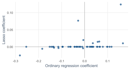
Shrinkage, coefficient by coefficient
The lasso keeps 12 of 51 predictors and shrinks even those.
Coefficients that make no sense
| Predictor | Ordinary regression | Lasso |
|---|---|---|
| semester 1 GPA | -0.03 | 0.08 |
| semester 2 GPA | 0.16 | 0.12 |
| semester 2 caffeine | 0.17 | 0.01 |
With 60 students, ordinary regression fits chance patterns. Shrunken coefficients cannot chase one sample’s noise.
Tuning penalty and mixture
glmnet_wf <- workflow(gpa_recipe,
  linear_reg(penalty = tune(), mixture = tune()) |> set_engine("glmnet"))

glmnet_grid <- expand_grid(penalty = 10^seq(-4, 0, length.out = 20),
                           mixture = c(0, 0.5, 1))

glmnet_tuning <- tune_grid(glmnet_wf, resamples = gpa_folds,
                           grid = glmnet_grid, metrics = metric_set(rmse))
20 penalties on a log scale, for ridge, an even elastic net, and lasso.
Too little, just right, too much
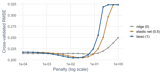
At the far right the lasso has zeroed every coefficient: back to the baseline. Best: mixture 1, penalty 0.013.
What the lasso keeps
best_penalty <- select_best(glmnet_tuning, metric = "rmse")
lasso_fit <- glmnet_wf |> finalize_workflow(best_penalty) |> fit(data = gpa_train)
tidy(lasso_fit) |> filter(estimate != 0) |> arrange(desc(abs(estimate)))
Of 51 predictors, the lasso keeps 10. Year-one GPA dominates.
One SD higher semester 2 GPA: about 0.15 points higher final GPA.
The lasso path
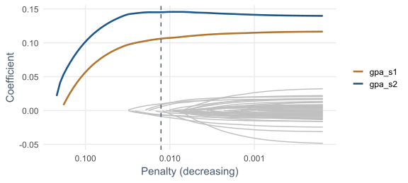
As the penalty falls, predictors enter one by one. The two GPA measures enter first.
Selected is not the same as causal
Sleep affects GPA (Chapter 8), yet the lasso drops it.
Its effect is already visible in year-one GPA, so it adds little to the prediction.
Among correlated predictors the lasso keeps one, and which one can change between samples. Predict with the lasso; explain with Chapters 8 and 10.
Boosting
flowchart LR
    A["Start:<br>the average"] --> B["Fit a small tree<br>to the errors"] --> C["Add it,<br>scaled down"]
    C -->|repeat hundreds of times| B
Each tree learns what the model so far missed. The learning rate keeps each step small.
Many weak trees add up to a strong model.
Boosting with one predictor
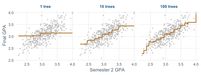
One step, a staircase, then a curve that follows the data.
Forests and boosting
| Random forest | Boosting | |
|---|---|---|
| trees grown | independently | in sequence |
| combined by | averaging | adding corrections |
| main settings | trees, mtry |
trees, learning rate, depth |
XGBoost is a fast, popular implementation, among the most successful methods for tables of data.
Tuning XGBoost
xgb_wf <- workflow(gpa_recipe,
  boost_tree(trees = 500, learn_rate = tune(), tree_depth = tune()) |>
    set_engine("xgboost") |> set_mode("regression"))

tune_grid(xgb_wf, resamples = gpa_folds,
          grid = expand_grid(learn_rate = c(0.01, 0.03, 0.1),
                             tree_depth = c(1, 2, 4)))
Best: depth 1, RMSE 0.212.
Depth-1 trees add separate effects with no interactions. Shallow winning means few interactions to find.
Comparing the models
| model | cross-validated RMSE | std. error |
|---|---|---|
| lasso | 0.204 | 0.009 |
| elastic net | 0.205 | 0.008 |
| XGBoost | 0.212 | 0.010 |
| ridge | 0.213 | 0.009 |
| linear regression | 0.218 | 0.010 |
| baseline (mean) | 0.323 | 0.010 |
Lasso and elastic net on top, XGBoost and ridge close behind, all better than ordinary regression. The differences are within a standard error; the lasso is chosen for using only 10 predictors.
The final test
final_lasso <- glmnet_wf |>
  finalize_workflow(best_penalty) |>
last_fit(gpa_split, metrics = regression_metrics)| MAE | RMSE | R² |
|---|---|---|
| 0.16 | 0.19 | 0.65 |
Off by 0.16 GPA points on average, capturing 65% of the variation.
Predicted against actual
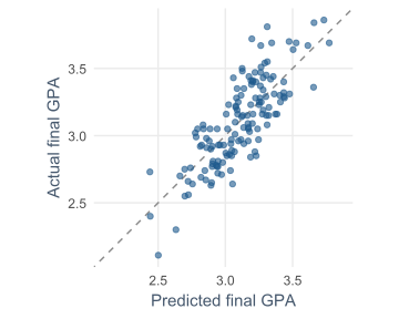
Predictions are less spread than reality: extreme students are pulled towards the average.
How much does year one add to past grades?
| Model | Test RMSE |
|---|---|
| lasso with everything | 0.192 |
| two year-one GPAs only | 0.193 |
Past grades are by far the best predictor. Sleep, stress, and support matter (Chapter 8), but their influence is already in the grades.
In your field: engineering
lm_concrete  <- workflow(compressive_strength ~ ., linear_reg())
xgb_concrete <- workflow(compressive_strength ~ .,
  boost_tree(trees = 500, learn_rate = 0.05, tree_depth = 4) |>
    set_engine("xgboost") |> set_mode("regression"))
Concrete strength from its recipe and age: curves and interactions.
Boosting cuts RMSE from 10.6 to 4.5 MPa. Flexible models win when the data has structure for them.
Practical lab: the Chapter 13 playground
Work through the playground exercises in your browser, with hints and solutions.
The browser version builds ridge regression by formula; the download uses glmnet and XGBoost.
Practical exercises 1–3: errors and shrinkage
- MAE and RMSE by hand; change one prediction by 1.0 and compare.
- Repeat the 60-student experiment with 150 students.
- Ridge against lasso coefficients: how many are exactly zero?
Practical exercises 4–6: design and communication
- Scale scores instead of 22 items: does the lasso’s RMSE change?
- XGBoost with 100, 500, and 1000 trees at learning rate 0.03.
- Explain an RMSE of 0.2 to academic advisers in two sentences.
Try this yourself
Take a prediction problem from your own field.
- count your cases and your predictors;
- name a baseline prediction;
- decide whether a lasso, a ridge, or boosting suits the structure;
- plan how you would report the final test.
Troubleshooting guide (Part 1)
| Symptom | Likely cause |
|---|---|
| near-perfect training fit, poor new predictions | too many predictors for the cases |
| coefficients huge and of opposite signs | multicollinearity |
| regularisation changes nothing | predictors not normalised |
| the lasso predicts the mean for everyone | penalty too large |
Troubleshooting guide (Part 2)
| Symptom | Likely cause |
|---|---|
| a different lasso selection each sample | correlated predictors; selection is unstable |
| the lasso “drops” a known cause | its effect is carried by another predictor |
| RMSE reported without a baseline | the number cannot be judged |
| extremes predicted too close to the mean | normal for imperfect models |
Completion checklist
Misconceptions to leave behind (Part 1)
| Misconception | Better mental model |
|---|---|
| more predictors always help | each is another chance to fit noise |
| the lasso’s predictors are what matters | they help prediction, chosen partly by chance |
Misconceptions to leave behind (Part 2)
| Misconception | Better mental model |
|---|---|
| a low RMSE means every prediction is accurate | extremes are pulled to the average |
| boosting always beats regression | only when curves and interactions exist |
The chapter in one sentence
With many predictors, shrink the coefficients or build from small trees, compare against a baseline by cross-validation, and never read a selected predictor as a cause.
Next: Chapter 14
The next chapter revisits clustering:
- what counts as a group;
- Gaussian mixture models and soft membership;
- clusters as dense regions: DBSCAN;
- evaluating a clustering;
- reporting the choices behind the clusters.
Questions
How many predictors, and how many cases, would your model have?
What is the simplest prediction your model must beat?