Advanced Clustering
Advanced Clustering
Every method carries a definition of what a group is
Chapter 14
Polla Fattah
By the end of today you can
- explain three definitions of a group;
- name the limits of k-means: hard assignments, round clusters, no outliers;
- fit a Gaussian mixture model, choose the number of clusters with BIC, and read membership probabilities;
- find dense clusters and noise points with DBSCAN, and choose its settings;
- evaluate a clustering with the silhouette, the adjusted Rand index, and interpretability.
Three definitions of a group
| A group is | Method | Allows |
|---|---|---|
| cases close to a common centre | k-means | nothing else |
| a population with its own distribution | Gaussian mixture model | partial membership |
| a dense region separated by sparse ones | DBSCAN | cases in no group |
The definition decides what the method can find.
Questions Chapter 9 left open
- how sure can we be which profile a student belongs to?
- is four really the right number?
- do some students fit no profile at all?
Same profile data: average habits across semesters, plus stress, support, satisfaction, scaled to z-scores.
Three assumptions of k-means
| Assumption | Problem |
|---|---|
| every case in exactly one cluster, with certainty | a student halfway between is assigned as firmly as one at the centre |
| clusters round and similar in size | elongated or unequal groups are cut wrongly |
| every case in some cluster | no way to say “fits nowhere” |
Real groups of people rarely satisfy these.
A simulation with known structure
shapes <- bind_rows(
  tibble(x = rnorm(100, 0, 0.4), y = rnorm(100, 0, 0.4), truth = "Round group"),
  tibble(x = rnorm(100, 3, 2),   y = rnorm(100, 1.4, 0.2), truth = "Long group"),
  tibble(x = runif(15, -2, 7),   y = runif(15, -2, 4),     truth = "Scattered"))

kmeans(xy, 2, nstart = 25)
Mclust(xy, G = 2)
dbscan(xy, eps = 0.5, minPts = 5)
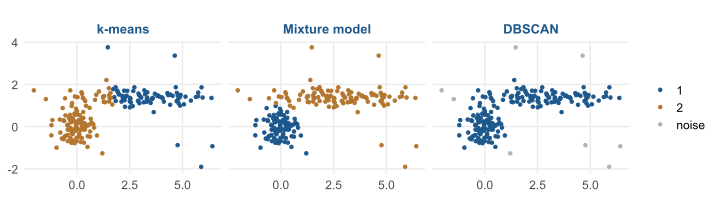
A round group, a long thin group, and 15 points that belong to neither.
Three methods, three answers
| k-means | mixture model | DBSCAN |
|---|---|---|
| ARI 0.53 | ARI 0.98 | ARI 0.00, and 6 of 15 scattered points as noise |
What each method saw
- k-means drew a straight boundary through the long group;
- the mixture model allowed the long group its elongated shape;
- DBSCAN joined the groups where they touch, one continuous dense region, but alone could say “no group”.
No method is right in general. Choose the definition deliberately, and state it.
Gaussian mixture models
The data is a mix of several groups, each with its own normal distribution.
The model estimates each group’s centre, spread, and size.
One variable: Old Faithful
| Short waits | Long waits | |
|---|---|---|
| mixing probability | 36% | 64% |
| mean (minutes) | 55 | 80 |
Mclust tried one to nine groups and chose 2.
Two normal curves over the data
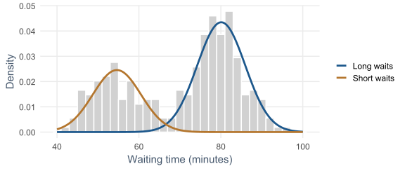
Waiting times between 272 eruptions: two humps, two groups.
Membership probabilities
| Wait | P(short) | P(long) |
|---|---|---|
| 50 minutes | 1 | 0 |
| 67 minutes | 0.42 | 0.58 |
| 85 minutes | 0 | 1 |
Not just which group, but how sure: soft assignments.
Shapes and BIC
With several variables, each group has a centre and a covariance matrix: round or elongated, tilted any way.
mclust names each shape with three letters, such as EEE (all equal) or VVV (all variable).
The Bayesian information criterion rewards fit and penalises parameters. In mclust, higher BIC is better.
Choosing the number of profiles
BIC chooses 3 clusters with the EVE structure.
The best four-cluster model is 8.7 BIC points behind: above 6 is strong evidence, above 10 very strong.
BIC by number of clusters
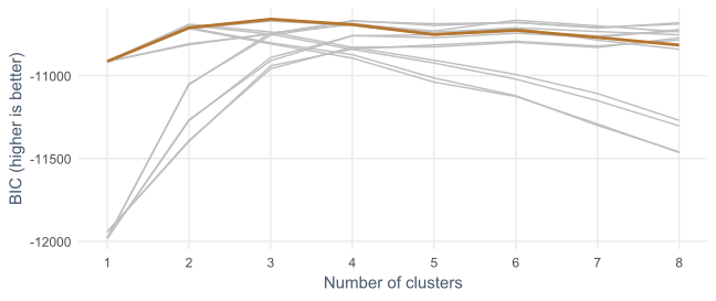
Each grey line is one covariance structure; the chosen one is copper.
Describing the three profiles
| cluster | students | sleep | study | caffeine | exercise | stress | support | satisfaction |
|---|---|---|---|---|---|---|---|---|
| 1 | 231 | 6.7 | 17.9 | 151.7 | 2.2 | 3.3 | 2.8 | 2.7 |
| 2 | 174 | 7.2 | 25.0 | 126.2 | 3.7 | 2.6 | 3.6 | 3.9 |
| 3 | 194 | 5.5 | 41.7 | 284.1 | 1.3 | 3.6 | 3.3 | 3.1 |
Balanced, overloaded, and disengaged or isolated. Cluster numbers are arbitrary labels.
Compared with k-means
- balanced and disengaged groups largely match;
- k-means’s two “overloaded” clusters are joined into one.
With flexible shapes, the mixture model did not need to split the overloaded students.
How certain is each assignment?
apply(..., 1, max) takes each row’s largest probability.
79 students have less than 80% probability for their most likely profile.
Uncertain students lie where profiles meet
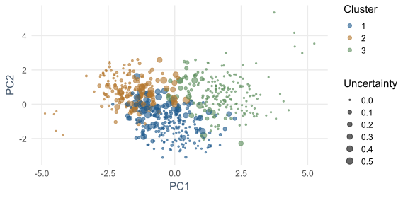
Report the share who clearly fit, and treat the rest as mixtures.
DBSCAN: clusters as dense regions
- a cluster is where cases are packed closely together;
- clusters are separated by sparser regions;
- cases in sparse regions are noise.
No number of clusters in advance, any shape, and “this case fits nowhere”.
Core points, border points, noise
| Setting or term | Meaning |
|---|---|
eps |
radius of each case’s neighbourhood |
minPts |
cases a neighbourhood needs to be dense |
| core point | at least minPts cases within eps |
| border point | near a core point, but not itself core |
| noise | everything else |
Core points within eps of each other join the same cluster.
A small example
tiny <- tibble(
  x = c(1.0, 1.2, 1.1, 0.9, 1.3,   4.0, 4.2, 3.9, 4.1, 4.3,   2.5, 5.5),
  y = c(1.0, 1.1, 1.3, 1.2, 0.9,   3.0, 3.2, 3.1, 2.8, 3.0,   4.5, 0.5))
dbscan(tiny, eps = 0.5, minPts = 3)$cluster
#>  [1] 1 1 1 1 1 2 2 2 2 2 0 0
Two tight groups become clusters 1 and 2; the two isolated points are 0, noise.
k-means would have had to put them into a group.
Choosing eps
Each student’s distance to their seventh-nearest neighbour, sorted.
The curve bends upward where isolated students begin: about 2. minPts = 8, roughly the number of variables plus one.
One cloud, a few outsiders
DBSCAN finds 1 cluster and 13 noise points.
Not a failure: students form one continuous cloud. The profiles are regions of that cloud, not separate islands.
Smaller eps breaks the cloud into fragments and labels hundreds as noise.
Students who fit no profile
| Kind | Pattern |
|---|---|
| extreme workers (5) | about 60 study hours, 4 hours’ sleep, over 700 mg caffeine, no exercise |
| extreme rest (5) | nearly 10 hours’ sleep, very little study or caffeine, exercise almost daily |
DBSCAN finds students unusual in their combination of values, not one variable at a time.
Keep them, report them separately, and check the profiles without them.
Evaluating a clustering
There are usually no true answers, so evaluation rests on several kinds of evidence:
| Evidence | Asks |
|---|---|
| internal measures | compact and well separated? |
| agreement between methods | do reasonable methods agree? |
| external validation | do clusters match known categories? |
| stability | do they survive small changes? |
| interpretability | do they make sense, and predict outcomes? |
Internal: the silhouette
profile_distances <- dist(profile_data)
mean(silhouette(kmeans_clusters$cluster, profile_distances)[, "sil_width"])
mean(silhouette(profile_gmm$classification, profile_distances)[, "sil_width"])| k-means | mixture model |
|---|---|
| 0.21 | 0.23 |
Both low on a −1 to 1 scale: the profiles overlap, as DBSCAN suggested.
The adjusted Rand index
first  <- c(1, 1, 1, 2, 2, 2)
second <- c("B", "B", "B", "A", "A", "A")
third  <- c(1, 1, 2, 2, 3, 3)
adjustedRandIndex(first, second)   #> 1
adjustedRandIndex(first, third)    #> much lower
Counts pairs put together or apart by both clusterings, adjusted for chance. Labels do not matter.
k-means against the mixture model: ARI 0.65, substantial agreement for four clusters against three.
Interpretability: do profiles predict outcomes?
| cluster | students | considering_dropout |
|---|---|---|
| 1 | 231 | 21% |
| 2 | 174 | 4% |
| 3 | 194 | 17% |
Dropout played no part in finding the profiles, yet they differ clearly on it.
Report the choices, not just the clusters
- which variables, and how they were scaled;
- which method, and why that definition of a group;
- how many clusters, with the evidence (BIC, silhouette);
- how clearly cases fit, such as the share above 0.8 probability;
- how robust the profiles are to other reasonable choices.
In your field: earth sciences
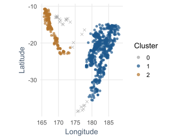
1,000 earthquakes near Fiji: DBSCAN follows the two curved trenches. Here dense regions really are separated by gaps.
Practical lab: the Chapter 14 playground
Work through the playground exercises in your browser, with hints and solutions.
The browser version uses a hand-written DBSCAN and ARI; the download uses mclust and dbscan.
Practical exercises 1–4: mixture models and DBSCAN
- Four mixture profiles: which three-cluster profile splits?
- How many students have a membership probability above 0.95?
- DBSCAN with
epsof 1.2, 1.6, and 2.4. - Refit the mixture model without the noise students.
Practical exercises 5–7: evaluation
- ARI between the mixture model and Ward’s hierarchical clustering.
- Compare the profiles on final GPA.
- Separate the simulated groups with a gap: what changes for each method?
Try this yourself
For grouping in your own field:
- which definition of a group fits your theory?
- would partial membership be meaningful?
- should some cases be allowed to fit no group?
- which outcome, not used to build the groups, could validate them?
Troubleshooting guide (Part 1)
| Symptom | Likely cause |
|---|---|
| an elongated group cut in two | k-means assumes round clusters |
| outliers forced into groups | k-means and mixtures place every case |
| BIC favours 3 and 4 almost equally | report both, with the evidence |
| lower BIC treated as better | in mclust, higher is better |
Troubleshooting guide (Part 2)
| Symptom | Likely cause |
|---|---|
| DBSCAN finds one cluster | a continuous cloud with no gaps |
| hundreds of noise points | eps too small |
| cluster labels differ between runs | labels are arbitrary; compare with ARI |
| low silhouette for every method | groups overlap; no clustering will be crisp |
Completion checklist
Misconceptions to leave behind (Part 1)
| Misconception | Better mental model |
|---|---|
| a sophisticated method finds the true groups | each finds groups matching its definition |
| every case belongs to some group | probabilities and noise describe reality better |
Misconceptions to leave behind (Part 2)
| Misconception | Better mental model |
|---|---|
| the best BIC proves the number of groups | nearby models may be almost as good |
| DBSCAN failed with one cluster | one continuous cloud is a finding |
The chapter in one sentence
Choose a definition of a group that fits your data, report how sure each assignment is and who fits nowhere, and judge clusters by agreement, stability, and meaning.
Next: Chapter 15
The next chapter introduces neural networks:
- a single neuron;
- from neurons to networks;
- a neural network for the dropout question;
- when neural networks are worth using;
- deep learning.
Questions
In your field, can a case belong partly to two groups?
What would a case that fits no group tell you?