Mixed-Effects Models
Mixed-Effects Models
When observations are not independent
Chapter 10
Polla Fattah
By the end of today you can
- recognise repeated-measures and nested data;
- explain, with a simulation, why ordinary regression gets their uncertainty wrong;
- fit random intercept and random slope models with lme4;
- interpret fixed effects, random effects, and the intraclass correlation;
- test whether an effect changes over time, and compare models;
- model a count outcome with a generalised linear mixed model;
- report a mixed-effects model in a thesis.
Two kinds of structure
| Structure | Example | Grouped within |
|---|---|---|
| repeated measures | four semesters per student | people |
| nested data | students with the same supervisor | groups |
Observations within a group are more alike than observations from different groups.
Less information than the rows suggest
A student who scores high this semester is likely to score high next semester.
Students of one supervisor share that supervisor’s style.
Methods that ignore this get the uncertainty wrong, sometimes badly.
A simulated training course with no effect
simulate_clustered <- function() {
  supervisor <- rep(1:20, each = 10)
  trained    <- rep(rep(c(0, 1), 10), each = 10)   # no real effect
  style      <- rnorm(20, sd = 5)[supervisor]      # shared by a supervisor's students
  wellbeing  <- 60 + style + rnorm(200, sd = 10)
  # ... test "trained" with lm() and with lmer()
}
20 supervisors, 10 students each, half the supervisors trained. Repeated 500 times.
Ignoring the grouping creates false alarms
| Analysis | Share of studies “significant” |
|---|---|
| ordinary regression | 27% |
| mixed-effects model | 7% |
| a correct test should give | 5% |
The course went to 20 supervisors, not 200 independent students.
The mixed model is slightly above 5% because the quick p-value ignores that there are only 20 supervisors.
A study of sleep deprivation
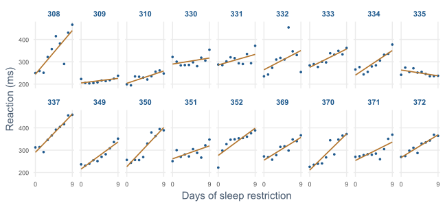
Reaction times of 18 people over 10 days of sleep restriction, one measurement per person per day.
180 rows, but only 18 people.
Everyone gets slower, but differently
People start at different levels (intercepts) and slow at different rates (slopes).
Random intercepts
(1 | Subject): one average line, but a separate starting level for each person.
Fixed and random effects
| Part | Describes | Here |
|---|---|---|
| fixed intercept | average reaction on day 0 | 251 ms |
| fixed slope | average change per day | 10.5 ms |
| SD of intercepts | how much people’s starting levels differ | 37 ms |
| residual SD | day-to-day variation within a person | 31 ms |
The intraclass correlation
\[ \text{ICC} = \frac{\text{variance between groups}}{\text{variance between groups} + \text{variance within groups}} \]
About 59% of the variation is stable differences between people.
ICC 0: the grouping does not matter. The higher it is, the more wrong an ordinary regression becomes.
Random slopes
(Days | Subject): a separate intercept and slope for each person.
| Random intercept | Random slope | |
|---|---|---|
| average slope | 10.5 ms | 10.5 ms |
| its standard error | 0.80 | 1.55 |
Slopes vary with SD ≈ 5.9 ms per day. Ignoring it made the average too confident.
Is the random slope worth it?
A likelihood ratio test compares the two models. The p-value is tiny: random slopes improve the model clearly.
AIC agrees: it balances fit against complexity, and lower is better.
The wellbeing panel
Up to four records per student, 2326 in all. time is 0 in semester 1.
Students differ far more than they change
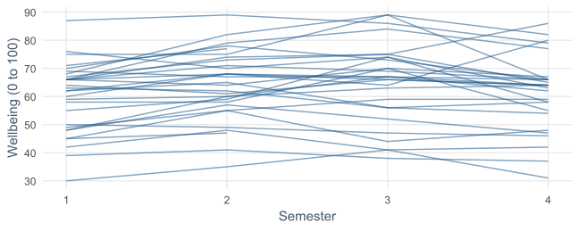
Thirty random students: each stays roughly at their own level.
The ICC for wellbeing
wb_null <- lmer(wellbeing ~ 1 + (1 | student_id), data = panel)
vc_null <- as.data.frame(VarCorr(wb_null))
vc_null$vcov[1] / sum(vc_null$vcov)
About 78% of all the variation in wellbeing lies between students.
The design effect
\[ \text{design effect} = 1 + (m - 1) \times \text{ICC} \]
| Value | |
|---|---|
| records | 2326 |
| design effect | 3.25 |
| independent equivalent | about 716 |
2326 records carry about as much information as 716 independent observations.
Does wellbeing decline? The wrong way
Slope -0.38, standard error 0.22: not significant.
The right way: a growth model
| Ordinary regression | Mixed model | |
|---|---|---|
| slope per semester | -0.38 | -0.43 |
| standard error | 0.22 | 0.11 |
The ordinary regression puts the large differences between students into its error, drowning the small change within each student.
The error can go either way
| Situation | Ignoring the structure |
|---|---|
| training course simulation | made a non-existent effect significant |
| sleep study slopes | made the average look too certain |
| wellbeing over time | made a real decline look uncertain |
The direction depends on the data. The error is always there.
lme4 prints no p-values
| Solution | How |
|---|---|
| confidence intervals | confint(wb_growth, parm = "beta_", method = "Wald") |
| likelihood ratio test | compare models with anova() |
| lmerTest | adds Satterthwaite p-values to summary() |
The time interval runs from -0.65 to -0.22: entirely below zero. Wellbeing declines, as RQ8 predicted.
lmerTest in practice
library(lmerTest)
wb_growth_p <- lmer(wellbeing ~ time + (time | student_id), data = panel)
summary(wb_growth_p)$coefficients
New columns: degrees of freedom and Pr(>|t|).
Models fitted after loading lmerTest include a p-value for each fixed effect.
Did the workshop effect last?
factor(semester) gives each semester its own average; the interaction lets the gap differ by semester.
Every record is used, including the first year of students who later left.
The effect fades
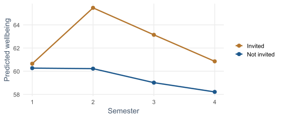
| Semester | 1 | 2 | 3 | 4 |
|---|---|---|---|---|
| gap (points) | 0.4 | 5.3 | 4.1 | 2.6 |
Predictions for the average student
predicted <- expand.grid(semester = 1:4,
                         workshop = c("Invited", "Not invited")) |>
  mutate(time = semester - 1)
predicted$wellbeing <- predict(wb_workshop, newdata = predicted,
                               re.form = NA)
re.form = NA ignores the random effects.
Every gap after semester 1 differs from the baseline gap (largest p = 0.001). A yearly follow-up session might keep the benefit going.
A singular fit
gpa_growth <- lmer(gpa ~ time + (time | student_id), data = panel)
#> boundary (singular) fit: see help('isSingular')
The model is more complex than the data supports: GPA slopes hardly vary.
Simplify to a random intercept only.
Grades stay stable
The slope of time is -0.000: almost exactly zero.
Wellbeing falls while grades hold. A non-change is a finding too.
Students within supervisors
| Level | Share of variation |
|---|---|
| between supervisors | 13% |
| between students, same supervisor | 65% |
| within students, over semesters | 22% |
Unique student IDs let R see the nesting. Who supervises a student makes a measurable difference.
Other outcomes: glmer()
| Outcome | Family | Coefficients become |
|---|---|---|
| yes or no | binomial |
odds ratios |
| counts | poisson |
rate ratios |
Supervisor meetings per semester are a count.
A count model for meetings
meetings_model <- glmer(
  supervisor_meetings ~ support + programme +
    (1 | supervisor_id) + (1 | student_id),
  data = panel |> left_join(support_scores, join_by(student_id)),
  family = poisson)
exp(fixef(meetings_model))
Each extra point of support: about 48% more meetings. PhD students: about 19% more.
The direction is uncertain: more meetings may also make students feel supported.
Mixed models and missing data
Students who left after year 1 were not a random group (Chapter 6).
Mixed models use every record each student gave, instead of dropping them.
The results hold as long as leaving depends on things the model can see: missing at random.
Reporting a mixed model
- the fixed effects, with confidence intervals;
- the random effects, as SDs or variance shares;
- the number of observations and of groups;
- which random effects were included.
Writing it up
A linear mixed-effects model with random intercepts and slopes for students (2326 observations of 600 students) showed that wellbeing declined by 0.43 points per semester (95% CI [0.22, 0.65]). Students differed considerably in their overall wellbeing (SD of intercepts = 10.7); 78% of the variation was between students.
In your field: agriculture
50 chicks weighed from birth to 21 days on four diets: repeated measurements in groups.
Diet 1: about 6.3 g a day. Diet 3 adds 5.1 g a day, 82% faster.
Practical lab: the Chapter 10 playground
Work through the playground exercises in your browser, with hints and solutions.
lme4 runs in the browser; every exercise also runs in RStudio.
Practical exercises 1–3: growth models
- A random intercept model for sleep over time: ICC and change.
- Add a random slope and compare with
anova(). - Does part-time students’ wellbeing change at a different rate?
Practical exercises 4–6: levels and simulation
- How much of the variation in study hours lies between supervisors?
- With supervisors who differ more, what happens to the false alarm rate?
- Explain to a fellow student why a regression of all semester records is wrong.
Try this yourself
Look at your own data for structure.
- is anyone measured more than once?
- do participants share a group: class, clinic, supervisor, site?
- estimate the ICC with a null model;
- calculate the design effect;
- decide which random effects your model needs.
Troubleshooting guide (Part 1)
| Symptom | Likely cause |
|---|---|
| effects significant that should not be | grouping ignored; standard errors too small |
| a real change not significant | between-person differences left in the error |
no p-values in summary() |
lme4 by design; use lmerTest or intervals |
| “boundary (singular) fit” | too many random effects for the data |
Troubleshooting guide (Part 2)
| Symptom | Likely cause |
|---|---|
| students not seen as nested | IDs repeated across supervisors |
| predictions differ per student | random effects included; use re.form = NA |
| Poisson coefficients hard to read | log scale; use exp() for rate ratios |
| later semesters look better | attrition; mixed models use all records |
Completion checklist
Misconceptions to leave behind (Part 1)
| Misconception | Better mental model |
|---|---|
| more rows means more evidence | grouped records repeat each other |
| ignoring grouping costs a little precision | it can multiply false alarms or hide effects |
Misconceptions to leave behind (Part 2)
| Misconception | Better mental model |
|---|---|
| averaging each person’s records solves it | it discards change and weights people unequally |
| a singular fit means the model is wrong | simplify the random effects |
The chapter in one sentence
When observations share a person or a group, model that structure: mixed models separate differences between groups from change within them and get the uncertainty right.
Next: Chapter 11
The next chapter turns from explanation to prediction:
- machine learning and generalisation;
- overfitting;
- a fair test with training and test data;
- cross-validation and tuning;
- the final test, and predictions about people.
Questions
What is the grouping structure in your own data?
How many truly independent units does your study have?