flowchart LR
  I1((Stress)) --> H1((H1))
  I1 --> H2((H2))
  I1 --> H3((H3))
  I2((Support)) --> H1
  I2 --> H2
  I2 --> H3
  I3((Sleep)) --> H1
  I3 --> H2
  I3 --> H3
  H1 --> O((P of<br>dropout))
  H2 --> O
  H3 --> O
Neural Networks
Neural Networks
Less mysterious than the reputation suggests
Chapter 15
Polla Fattah
By the end of today you can
- explain how a neuron combines its inputs;
- explain why a single sigmoid neuron is a logistic regression;
- describe layers, weights, activation functions, and training;
- fit and tune a network with
mlp(), using weight decay; - compare a network fairly with simpler models;
- say when deep learning is, and is not, the right tool.
A claim worth testing
“A neural network would surely predict better than logistic regression.”
Neural networks power image recognition, speech, translation, and large language models.
On a table of research data, the claim should be tested, not accepted.
A single neuron
| Step | Does |
|---|---|
| weight | multiplies each input |
| bias | a constant added to the total |
| activation function | turns the total into the output |
Two inputs, stress and support, with weights 1.2 and −0.8, and a bias of −4.
Working one neuron by hand
For a student with stress 4 and support 2:
\[ -4 + 1.2 \times 4 - 0.8 \times 2 = -0.8 \]
The sigmoid squeezes any number into 0 to 1:
\[ \text{sigmoid}(z) = \frac{1}{1 + e^{-z}} \]
The neuron in R
A single neuron is a logistic regression
| Neuron | Logistic regression (Chapter 8) |
|---|---|
| bias | intercept |
| weights | coefficients |
| sigmoid | turns log odds into a probability |
Everything a single neuron can do, Chapter 8 has already done.
From neurons to networks
A multilayer perceptron: inputs, a hidden layer, an output. Every arrow is a weight.
Why layers add power
- each hidden neuron learns its own combination of inputs;
- the output neuron combines those;
- curved activations let the network represent curves and interactions.
With enough hidden neurons, a network can approximate almost any relationship. That flexibility is its strength, and its danger.
Two activation functions
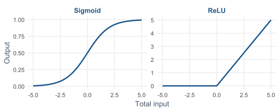
The sigmoid squeezes into 0 to 1. The ReLU zeroes negatives and is standard in deep networks.
How a network learns
- start with small random weights;
- for every weight, find whether a small change would reduce the error: the gradient;
- move all weights a little in the helpful direction: gradient descent;
- one pass through the data is an epoch; training runs for hundreds.
Six students, one neuron
Stress is measured from the group’s average.
The error to reduce is the log loss: small when high probabilities go to students who did consider dropping out.
Starting from zero
log_loss <- function(b0, b1) {
  p <- sigmoid(b0 + b1 * six$stress)
  -mean(six$dropout * log(p) + (1 - six$dropout) * log(1 - p))
}
log_loss(0, 0)   #> 0.693
With both weights at zero, every student gets a probability of 0.5.
The gradient
p <- sigmoid(b0 + b1 * six$stress)
gradient_b0 <- mean(p - six$dropout)
gradient_b1 <- mean((p - six$dropout) * six$stress)
The average prediction error, multiplied by the weight’s input (1 for the bias).
The stress gradient is -0.292: negative, so increasing the weight would reduce the error.
One step of gradient descent
| Before | After one step | |
|---|---|---|
| stress weight | 0 | 0.292 |
| log loss | 0.693 | 0.616 |
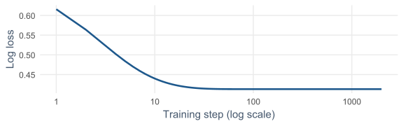
Training is nothing more than this step, repeated.
2,000 steps
| Bias | Stress weight | |
|---|---|---|
| gradient descent | 0.000 | 2.428 |
glm() |
0.000 | 2.428 |
Two consequences
- training starts from random weights, so two runs differ:
set.seed()matters; - many weights can keep reducing training error by memorising noise.
Weight decay penalises large weights, exactly like the ridge penalty of Chapter 13. In tidymodels it is penalty.
Backpropagation calculates gradients efficiently for thousands of weights.
A network for the dropout question
mlp(hidden_units = , penalty = , epochs = ) |>
  set_engine("nnet", MaxNWts = 5000) |>
  set_mode("classification")
Same data, split, recipe, and folds as Chapters 11 and 12. Networks need normalised inputs; the recipe provides them.
The nnet engine, which comes with R, fits one hidden layer.
A network that memorises
big_net <- mlp(hidden_units = 20, penalty = 0, epochs = 1000) |>
  set_engine("nnet", MaxNWts = 5000) |> set_mode("classification")
big_fit <- fit(workflow(dropout_recipe, big_net), data = dropout_train)| Data | AUC |
|---|---|
| training | 1.00 |
| test | 0.64 |
521 weights for 449 students: more than enough freedom to memorise every one.
Tuning size and weight decay
net_spec <- mlp(hidden_units = tune(), penalty = tune(), epochs = 500) |>
  set_engine("nnet", MaxNWts = 5000) |> set_mode("classification")

net_grid <- expand_grid(hidden_units = c(1, 3, 5, 10, 20),
                        penalty = 10^seq(-2, 1.5, by = 0.5))
Weight decay on a log scale from 0.01 to about 30.
The penalty matters more than the size
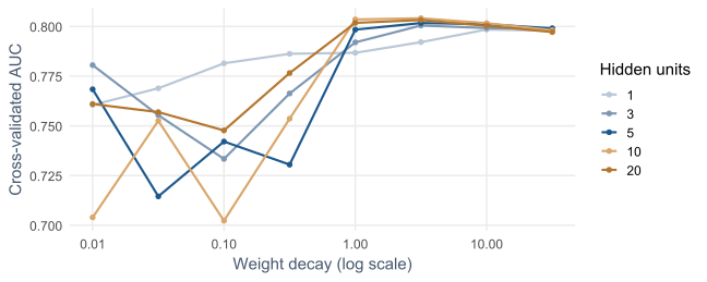
Little decay: networks overfit, the big ones most. Enough decay: every size does about equally well.
A fair comparison
| Model | Cross-validated AUC | Test AUC |
|---|---|---|
| tuned network (10 hidden units) | 0.804 | 0.85 |
| logistic regression | 0.804 | 0.84 |
With 151 test students, 23 at risk, this difference is well within chance.
A neural network does not predict dropout better.
The costs of the network
- 261 weights that cannot be interpreted: no odds ratios;
- results depend on random starting weights without strong decay;
- careful tuning needed to avoid overfitting.
Logistic regression is kept. Reporting that a network was tried and did not help is itself a finding.
When neural networks are worth using
| Situation | Why networks help |
|---|---|
| unstructured data: images, sound, text | features must be learned from raw inputs |
| very large datasets | thousands of weights need many cases |
| complex non-linear relationships | flexibility finds structure |
A table of a few hundred cases and a few dozen variables, the typical thesis, rarely qualifies.
Deep learning
- many hidden layers, millions or billions of weights;
- each layer builds on the last: edges, then shapes, then objects;
- convolutional networks for images, transformers for text;
- large language models (Chapter 18) are transformers with billions of weights.
Deep learning in R
| Tool | Notes |
|---|---|
| keras3 | interface to Keras; needs Python alongside R |
| torch | the PyTorch engine, without Python |
| brulee | tidymodels deep networks through torch, with mlp() |
For most researchers, the practical route is a pretrained model, as Chapter 18 does with a language model.
In your field: engineering
concrete_recipe <- recipe(compressive_strength ~ ., data = training(concrete_split)) |>
  step_log(age) |>
  step_normalize(all_numeric_predictors())
concrete_net <- mlp(hidden_units = 10, penalty = 0.1, epochs = 1000) |>
set_engine("nnet", MaxNWts = 5000) |> set_mode("regression")| Model | Test RMSE (MPa) |
|---|---|
| linear regression | 7.2 |
| neural network | 5.0 |
Curves and interactions give the flexibility something to capture.
Practical lab: the Chapter 15 playground
Work through the playground exercises in your browser, with hints and solutions.
nnet runs in the browser; the download uses tidymodels.
Practical exercises 1–3: neurons and networks
- Double the importance of support in the neuron: what does a negative weight mean?
- One hidden neuron with decay 1 against logistic regression.
- Three seeds with decay 0.01 and with the best decay: when does the seed matter?
Practical exercises 4–6: training
- The 20-neuron network for 10, 100, and 1000 epochs.
- Explain to the research group why the thesis keeps logistic regression.
- Gradient descent with learning rates 0.1 and 10: what goes wrong?
Try this yourself
Someone suggests “just use AI” for your prediction problem.
- how many cases and variables do you have?
- is the data a table, or images, sound, or text?
- what simple model would you compare against?
- what would you lose in interpretability?
Troubleshooting guide (Part 1)
| Symptom | Likely cause |
|---|---|
| perfect training AUC | memorisation; add weight decay |
| different results on each run | random starting weights; set a seed, add decay |
| “too many weights” error | raise MaxNWts |
| a network no better than regression | a smooth pattern; that is a finding |
Troubleshooting guide (Part 2)
| Symptom | Likely cause |
|---|---|
| loss explodes during training | learning rate too large |
| loss barely moves | learning rate too small, or too few epochs |
| inputs on very different scales | missing step_normalize() |
| no one can explain the model | many uninterpretable weights |
Completion checklist
Misconceptions to leave behind (Part 1)
| Misconception | Better mental model |
|---|---|
| a neural network is always more accurate | on typical tables, often not |
| networks learn mysteriously | gradient descent: small steps that reduce error |
Misconceptions to leave behind (Part 2)
| Misconception | Better mental model |
|---|---|
| a perfect training fit means learning | usually memorisation |
| neural networks and AI are the same | networks are one family; LLMs are one kind |
The chapter in one sentence
A neural network is logistic regression units stacked in layers and trained by small steps; it earns its complexity on large, unstructured, or strongly non-linear data, not on every table.
Next: Chapter 16
The next chapter turns to data ordered in time:
- time series data and its components;
- the counselling service’s weekly visits;
- decomposition into trend and seasonality;
- forecasting, and judging forecasts;
- what forecasts assume about the future.
Questions
What would convince you that a neural network is worth its cost?
What would you report if it were not?