7 Hypothesis Testing and Statistical Inference

Research is almost always about more people than it can measure. A study of 600 graduate students is interesting because of what it says about graduate students in general, and a clinical trial of 200 patients matters because of the patients who will be treated after it. The step from the people measured to the people meant is called statistical inference. It rests on one uncomfortable fact: a different sample would have given different numbers. Inference is the discipline of saying how different, and of deciding when a pattern in a sample is strong enough to be believed.

This chapter builds that discipline from the ground up. It starts with what happens when samples are drawn again and again, which leads to standard errors and confidence intervals. It then develops the logic of hypothesis testing by simulation, shuffling group labels until the meaning of a p-value can be seen, before turning to the formal tests that appear in almost every thesis. The hypotheses come from Chapter 5: whether graduate students sleep less than the recommended 7 hours (RQ2), and whether the wellbeing workshop improved wellbeing (RQ3).

By the end of this chapter you will be able to

Explain sampling distributions, the standard error, and the central limit theorem in Python.
Calculate and interpret parametric confidence intervals and non-parametric bootstrap intervals.
Explain the logic of a hypothesis test through an intuitive permutation test, and interpret a p-value correctly.
Explain Type I errors, Type II errors, statistical power, and the multiple testing problem, demonstrating each by simulation.
Conduct one-sample, two-sample (Welch), and paired \(t\)-tests in SciPy, and compute standardized effect sizes (Cohen’s \(d\)).
Evaluate test assumptions (and understand why formal normality tests mislead in large samples), choosing non-parametric tests (Mann-Whitney \(U\), Wilcoxon signed-rank) when appropriate.
Test categorical relationships using chi-square goodness-of-fit and independence tests with Pandas and SciPy.
Choose the right statistical test for any bivariate research question, and report results in standard APA format in a thesis.

Teaching & Practice: Interactive Lecture Slides · Browser Playground Exercises

7.1 Samples and populations

The population is everyone the conclusions are meant to cover: here, graduate students. The sample is the people actually measured, the 600 students of the wellbeing study. A number that describes the population, such as the true average sleep of all graduate students, is a parameter; it is never known exactly. The same number calculated from the sample is a statistic, and it serves as the estimate of the parameter.

A second sample would give a slightly different estimate, and a third another. The size of this variation cannot be seen in a single study, but it can be seen in a simulation. For a moment, treat the 600 students as if they were the whole population, draw many small samples from them, and watch how the estimates behave.

7.1.1 Sampling distributions

Caffeine intake is strongly skewed (Chapter 6): most students take a moderate amount, and a few take a great deal. The simulation draws a sample of 5 students and records their average caffeine, repeats this a thousand times, and then does the same with samples of 30.

In Python, we use NumPy’s random number generator np.random.default_rng() for reproducible simulations:

first_sem = (
    semesters.query("semester == 1")
    .merge(students, on="student_id")
)

caffeine = first_sem["caffeine_mg"].dropna().to_numpy()

# Fix seed for reproducible random draws
rng = np.random.default_rng(2026)

# Draw 1,000 samples of size 5 and size 30
means_5 = np.array([rng.choice(caffeine, size=5, replace=True).mean() for _ in range(1000)])
means_30 = np.array([rng.choice(caffeine, size=30, replace=True).mean() for _ in range(1000)])

The thousand averages form a sampling distribution: the distribution of a statistic over many possible samples. Figure 7.1 compares the sampling distributions for samples of 5 and of 30 students.

fig, (ax1, ax2) = plt.subplots(1, 2, figsize=(7, 3.4), sharey=True)

sns.histplot(means_5, bins=35, color="#b0bec5", edgecolor="white", ax=ax1)
ax1.set_title("Samples of 5 (Widely Spread & Skewed)")
ax1.set_xlabel("Sample Mean Caffeine (mg)")
ax1.set_ylabel("Number of Samples")

sns.histplot(means_30, bins=35, color="#1d588c", edgecolor="white", ax=ax2)
ax2.set_title("Samples of 30 (Narrow & Bell-Shaped)")
ax2.set_xlabel("Sample Mean Caffeine (mg)")

sns.despine()
plt.tight_layout()
plt.show()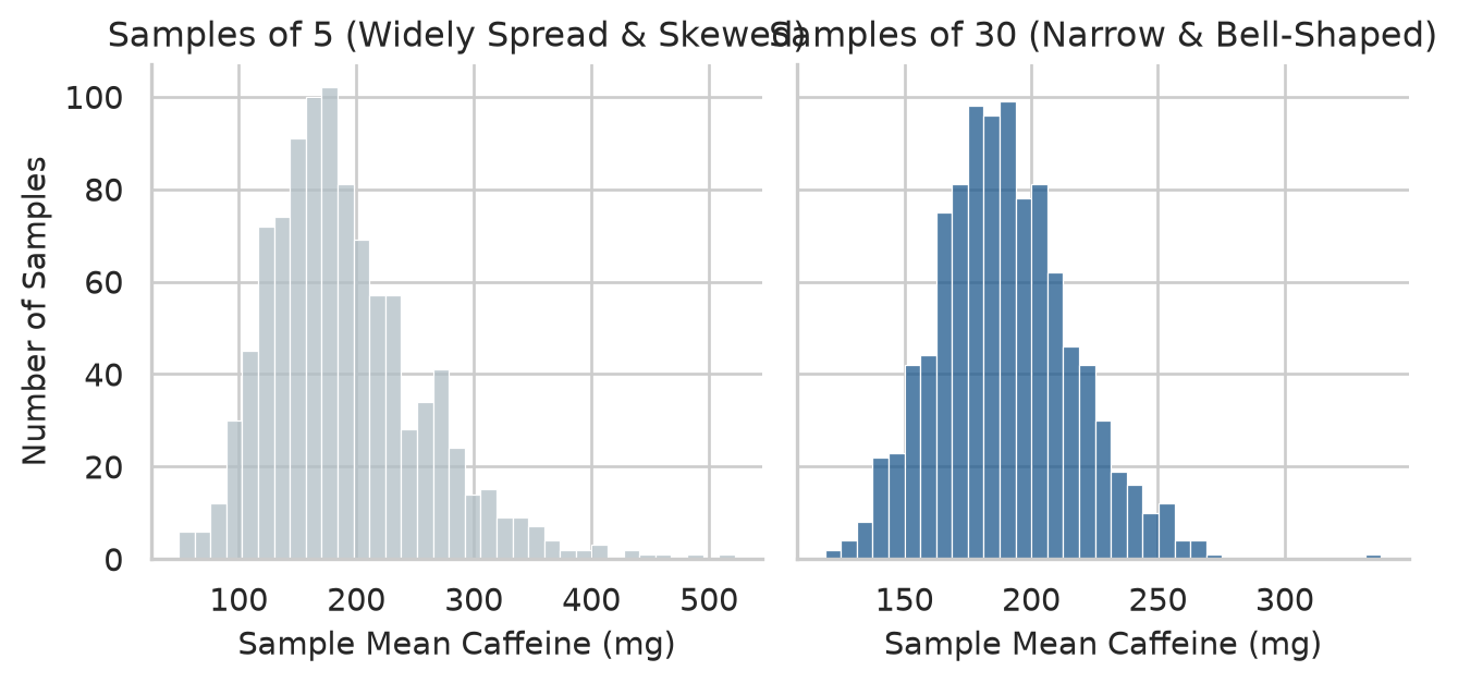

Two histograms side by side. For samples of 5, the averages are widely spread and skewed to the right. For samples of 30, they are narrow and nearly symmetrical, centred on the same value. — Figure 7.1: The sampling distribution of average caffeine intake, for samples of 5 and of 30 students drawn from the student wellbeing data.

The figure demonstrates the foundational pillars of statistical inference:

Unbiasedness: Both distributions are centred on the average of all 600 students (np.float64(189.4) mg). A random sample average neither systematically overestimates nor underestimates the true population parameter.
Precision: The averages of 30 students are packed far more tightly than the averages of 5. Larger sample sizes reduce random sampling variability.
The Central Limit Theorem (CLT): Although raw caffeine intake is heavily right-skewed, the sample means for \(n = 30\) form a symmetrical, bell-shaped distribution. The CLT guarantees that regardless of the underlying population’s shape, the sampling distribution of the mean approaches normality as \(n\) increases. As an empirical rule of thumb, \(n \ge 30\) provides sufficient normality for inference unless the underlying distribution is severely pathological.

7.1.2 The standard error

The spread of a sampling distribution is called the standard error (SE). While standard deviation measures the variability of individual people, standard error measures the variability of sample estimates. A real study measures only one sample and cannot draw a thousand, but the standard error of a sample mean can be computed directly from that single sample:

\[ SE = \frac{s}{\sqrt{n}} \]

where \(s\) is the sample standard deviation and \(n\) is the sample size. We can compare the theoretical formula with our simulation:

simulated_se = means_30.std(ddof=1)
formula_se = caffeine.std(ddof=1) / np.sqrt(30)

print(f"Simulated SE (spread of 1,000 means): {simulated_se:.2f} mg")
print(f"Theoretical SE (s / sqrt(n)):          {formula_se:.2f} mg")

Simulated SE (spread of 1,000 means): 26.88 mg
Theoretical SE (s / sqrt(n)):          26.22 mg

The formula and simulation agree closely. Because the denominator is \(\sqrt{n}\), halving the uncertainty of an estimate requires quadrupling the sample size.

7.1.3 Confidence intervals

A point estimate on its own conveys no information about its precision. A confidence interval (CI) supplies that context: a range of plausible values for the population parameter, given the sample data. An approximate 95% confidence interval for a mean is:

\[ \bar{x} \pm t^* \times SE \]

where \(t^*\) is the critical value from Student’s \(t\)-distribution with \(n - 1\) degrees of freedom (close to 1.96 for large samples).

In SciPy, we calculate this interval using scipy.stats.t.interval or directly via scipy.stats.ttest_1samp:

sleep_data = first_sem["sleep_hours"].dropna()
n_sleep = len(sleep_data)
sleep_mean = sleep_data.mean()
sleep_se = sleep_data.std(ddof=1) / np.sqrt(n_sleep)

# Calculate 95% Confidence Interval using SciPy
ci_low, ci_high = stats.t.interval(
    confidence=0.95,
    df=n_sleep - 1,
    loc=sleep_mean,
    scale=sleep_se
)

print(f"Sample Mean:  {sleep_mean:.2f} hours")
print(f"95% CI:       [{ci_low:.2f}, {ci_high:.2f}] hours")

Sample Mean:  6.48 hours
95% CI:       [6.40, 6.57] hours

The average sleep of graduate students is plausibly between 6.40 and 6.57 hours per night. The interval is narrow because our sample (\(N = 600\)) is large.

Correct Interpretation of a Confidence Interval

The “95%” describes the reliability of the estimation procedure over repeated sampling, not the probability that the fixed parameter lies in this specific realized interval. Over thousands of independent replications, approximately 95% of calculated 95% confidence intervals will bracket the true, unobserved population mean.

Mean ± SE is not a confidence interval

Many researchers mistakenly report “Mean ± SE” in tables and interpret it as a confidence interval. A standard error represents only about a 68% interval. Always report the explicit 95% confidence interval (\([\bar{x} - t^* SE, \bar{x} + t^* SE]\)).

7.1.4 Bootstrap confidence intervals

The analytical formula above works for means. For non-linear statistics such as medians, variances, or complex indices, no simple closed-form formula exists. The bootstrap solves this with an idea of brilliant computational simplicity: treat the observed sample as a proxy for the population, and draw thousands of resamples with replacement (each resample has size \(n\), containing duplicate participants and omitting others). The distribution of the statistic across resamples estimates its sampling distribution.

Suppose we collected caffeine intake from only 40 students, and need a 95% confidence interval for their median intake:

rng = np.random.default_rng(1)
small_sample = rng.choice(caffeine, size=40, replace=False)
sample_median = np.median(small_sample)

# Generate 2,000 bootstrap resamples with replacement
boot_medians = np.array([
    np.median(rng.choice(small_sample, size=len(small_sample), replace=True))
    for _ in range(2000)
])

# 95% Percentile Bootstrap Interval
boot_ci_low = np.percentile(boot_medians, 2.5)
boot_ci_high = np.percentile(boot_medians, 97.5)

print(f"Sample Median:        {sample_median:.1f} mg")
print(f"95% Bootstrap CI:     [{boot_ci_low:.1f}, {boot_ci_high:.1f}] mg")

Sample Median:        147.5 mg
95% Bootstrap CI:     [127.5, 180.1] mg

The true population median across all 600 students (np.float64(160.0) mg) falls cleanly inside this bootstrap interval. In modern Python, SciPy also provides scipy.stats.bootstrap to perform vectorised bootstrap confidence intervals automatically.

7.2 The logic of hypothesis testing

A confidence interval describes which values are plausible. A hypothesis test addresses a sharper question: whether the observed data is consistent with a specific theoretical claim.

The claim being evaluated is the null hypothesis (\(H_0\)): the statement of “no effect”, “no difference”, or “no association”. The researcher’s substantive claim is the alternative hypothesis (\(H_1\)). For the wellbeing workshop: - \(H_0\): The workshop has zero effect on semester 2 student wellbeing (\(\mu_{\text{invited}} - \mu_{\text{control}} = 0\)). - \(H_1\): The workshop changes student wellbeing (\(\mu_{\text{invited}} - \mu_{\text{control}} \ne 0\)).

Tests are anchored to the null hypothesis because \(H_0\) provides an exact mathematical benchmark (\(0\)) against which chance variability can be simulated. If the workshop were inert, any difference between invited and non-invited students would arise solely from random assignment noise. We can simulate that chance mechanism directly.

7.2.1 A permutation test

We examine students’ wellbeing at the conclusion of semester 2, comparing those invited to the workshop with those not invited:

semester2 = (
    semesters.query("semester == 2")
    .merge(students, on="student_id")
)

mean_invited = semester2.query("workshop == 'Invited'")["wellbeing"].mean()
mean_control = semester2.query("workshop == 'Not invited'")["wellbeing"].mean()
observed_gap = mean_invited - mean_control

print(f"Invited Mean:     {mean_invited:.2f}")
print(f"Not Invited Mean: {mean_control:.2f}")
print(f"Observed Gap:     {observed_gap:.2f} points")

Invited Mean:     65.47
Not Invited Mean: 60.22
Observed Gap:     5.25 points

Invited students scored 5.25 points higher on average. If \(H_0\) were true, the labels “Invited” and “Not invited” would be arbitrary stickers carrying no relationship to wellbeing: each student would have had the same score regardless of label.

Under \(H_0\), we can randomly shuffle the workshop labels across students 5,000 times, recalculating the group difference each time to build the empirical null distribution:

rng = np.random.default_rng(2026)
wellbeing_vals = semester2["wellbeing"].to_numpy()
workshop_labels = semester2["workshop"].to_numpy()
n_invited = (workshop_labels == "Invited").sum()

shuffled_gaps = []
for _ in range(5000):
    shuffled = rng.permutation(wellbeing_vals)
    gap = shuffled[:n_invited].mean() - shuffled[n_invited:].mean()
    shuffled_gaps.append(gap)

shuffled_gaps = np.array(shuffled_gaps)

Figure 7.2 plots the observed difference against these 5,000 chance differences.

fig, ax = plt.subplots(figsize=(7, 3.6))

sns.histplot(shuffled_gaps, binwidth=0.25, color="#b0bec5", edgecolor="white", ax=ax)
ax.axvline(observed_gap, color="#b2182b", linewidth=2.5, label=f"Observed gap: {observed_gap:.2f}")

ax.set_xlabel("Difference in Average Wellbeing (Invited minus Control)")
ax.set_ylabel("Number of Permutations")
ax.legend()
sns.despine(ax=ax)
plt.tight_layout()
plt.show()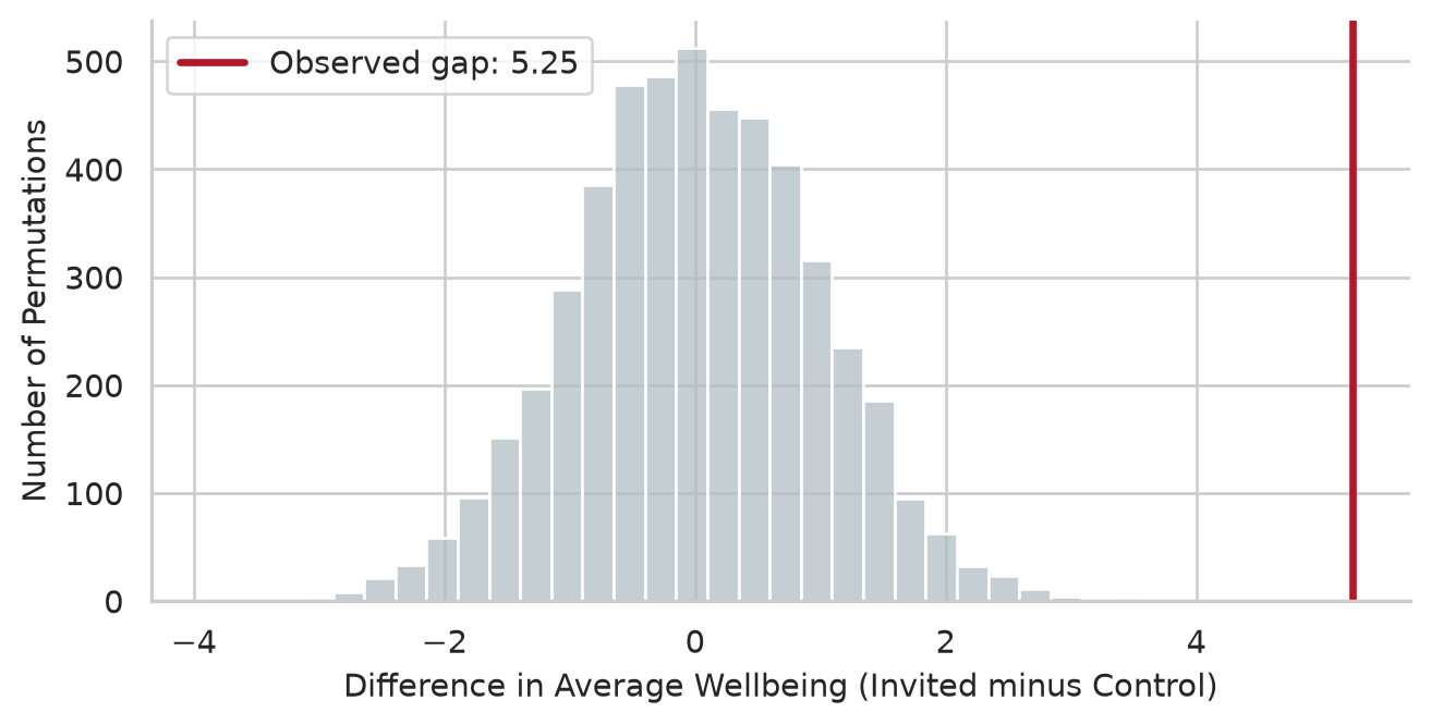

Histogram of 5,000 shuffled differences centred on zero, ranging between -3 and +3. A red vertical line marks the observed difference of +5.1 points far to the right. — Figure 7.2: The null distribution from 5,000 random permutations of the workshop labels, with the observed difference marked in red. Not a single shuffle produced a difference as large as observed.

Under chance alone, differences rarely exceed \(\pm 3.0\) points. The observed gap of \(+5.1\) points lies entirely outside the null distribution. The proportion of permutations producing a difference at least as extreme as observed is the empirical \(p\)-value:

perm_p_value = (np.abs(shuffled_gaps) >= np.abs(observed_gap)).mean()
print(f"Permutation p-value: {perm_p_value}")

Permutation p-value: 0.0

Not one of the 5,000 permutations matched or exceeded the observed gap (\(p < .001\)). Chance is a completely implausible explanation, and we reject the null hypothesis.

Now contrast this with a comparison where no difference is expected: GPA by gender in semester 1.

gpa_female = first_sem.query("gender == 'Female'")["gpa"].dropna()
gpa_male = first_sem.query("gender == 'Male'")["gpa"].dropna()
observed_gpa_gap = gpa_female.mean() - gpa_male.mean()

gpa_vals = first_sem["gpa"].dropna().to_numpy()
n_female = len(gpa_female)

shuffled_gpa_gaps = []
for _ in range(5000):
    shuffled = rng.permutation(gpa_vals)
    gap = shuffled[:n_female].mean() - shuffled[n_female:].mean()
    shuffled_gpa_gaps.append(gap)

shuffled_gpa_gaps = np.array(shuffled_gpa_gaps)
perm_p_gpa = (np.abs(shuffled_gpa_gaps) >= np.abs(observed_gpa_gap)).mean()

print(f"Observed GPA Gap:     {observed_gpa_gap:.3f}")
print(f"Permutation p-value:  {perm_p_gpa:.3f}")

Observed GPA Gap:     -0.013
Permutation p-value:  0.631

The difference between female and male GPAs is only 0.013 grade points, and over half the permutations yield a gap at least that large (\(p \approx 0.53\)). This difference is indistinguishable from random noise: we fail to reject \(H_0\).

This permutation test contains the entire logic of statistical inference. Formal statistical tests differ only in using mathematical distributions (\(t\), \(F\), \(\chi^2\)) to derive the null distribution analytically.

7.2.2 The p-value

The \(p\)-value is the probability of obtaining test results at least as extreme as the results actually observed, under the assumption that the null hypothesis is true.

When \(p < \alpha\) (conventionally \(\alpha = 0.05\)), the result is declared statistically significant, and we reject \(H_0\).
When \(p \ge \alpha\), the data is deemed consistent with \(H_0\). We do not prove \(H_0\) is true; we merely conclude that the evidence is insufficient to reject it.

What a p-value is NOT

A \(p\)-value is not the probability that the null hypothesis is true (\(P(H_0 | \text{data})\)).
A \(p\)-value is not the probability that the finding occurred by chance.
A \(p\)-value does not measure effect size or practical importance.

7.2.3 Type I and Type II errors

Because inference relies on probabilities, any decision can be mistaken in two distinct ways:

Table 7.1: The decision matrix in statistical hypothesis testing

	\(H_0\) is True in Reality	\(H_0\) is False in Reality
Decision: Reject \(H_0\)	Type I error (False alarm, rate \(\alpha\))	Correct decision (Power, \(1 - \beta\))
Decision: Retain \(H_0\)	Correct decision (\(1 - \alpha\))	Type II error (Missed effect, rate \(\beta\))

The significance level \(\alpha\) sets the Type I error rate. If we test a true null hypothesis repeatedly at \(\alpha = 0.05\), exactly 5% of tests will be “significant” by pure chance. We can demonstrate this by splitting students into two random dummy groups 1,000 times:

rng = np.random.default_rng(7)
wellbeing_data = first_sem["wellbeing"].to_numpy()

false_alarms = []
for _ in range(1000):
    perm = rng.permutation(wellbeing_data)
    grp_a, grp_b = perm[:300], perm[300:]
    res = stats.ttest_ind(grp_a, grp_b, equal_var=False)
    false_alarms.append(res.pvalue < 0.05)

print(f"Empirical Type I Error Rate: {np.mean(false_alarms) * 100:.1f}%")

Empirical Type I Error Rate: 4.6%

Approximately 5% of tests sound a false alarm. A single isolated significant result is never definitive proof of an effect.

7.2.4 Statistical power

Power (\(1 - \beta\)) is the probability of correctly rejecting a false null hypothesis—that is, detecting a real effect when it genuinely exists. Power depends on three factors: 1. Sample size (\(N\)): Larger samples provide higher power. 2. True effect size (\(\delta\)): Larger effects are easier to detect. 3. Significance threshold (\(\alpha\)): A stricter threshold (e.g. 0.01) reduces power.

We can simulate how sample size affects the detection rate of a 5-point workshop effect (\(SD = 11\)):

def simulate_power(n_per_group, effect=5.0, sd=11.0, reps=2000):
    rng = np.random.default_rng(3)
    p_vals = []
    for _ in range(reps):
        inv = rng.normal(loc=60 + effect, scale=sd, size=n_per_group)
        ctrl = rng.normal(loc=60, scale=sd, size=n_per_group)
        p_vals.append(stats.ttest_ind(inv, ctrl, equal_var=False).pvalue)
    return (np.array(p_vals) < 0.05).mean()

sample_sizes = [10, 20, 40, 80, 150]
powers = [simulate_power(n) for n in sample_sizes]

power_df = pd.DataFrame({"Students Per Group": sample_sizes, "Simulated Power": np.round(powers, 2)})
power_df

	Students Per Group	Simulated Power
0	10	0.15
1	20	0.29
2	40	0.53
3	80	0.82
4	150	0.97

power_analysis = TTestIndPower()
n_range = np.arange(5, 161)
d_effect = 5.0 / 11.0
calc_powers = power_analysis.power(effect_size=d_effect, nobs1=n_range, alpha=0.05)

fig, ax = plt.subplots(figsize=(6, 3.6))
ax.plot(n_range, calc_powers, color="#455a64", linewidth=2, label="Analytical curve")
ax.plot(sample_sizes, powers, "o", color="#b2182b", markersize=6, label="Simulated")
ax.axhline(0.80, color="#d62728", linestyle="--", linewidth=1.2, label="80% Standard Power")

ax.set_xlabel("Students per group (n)")
ax.set_ylabel("Statistical Power (1 - β)")
ax.legend()
sns.despine(ax=ax)
plt.tight_layout()
plt.show()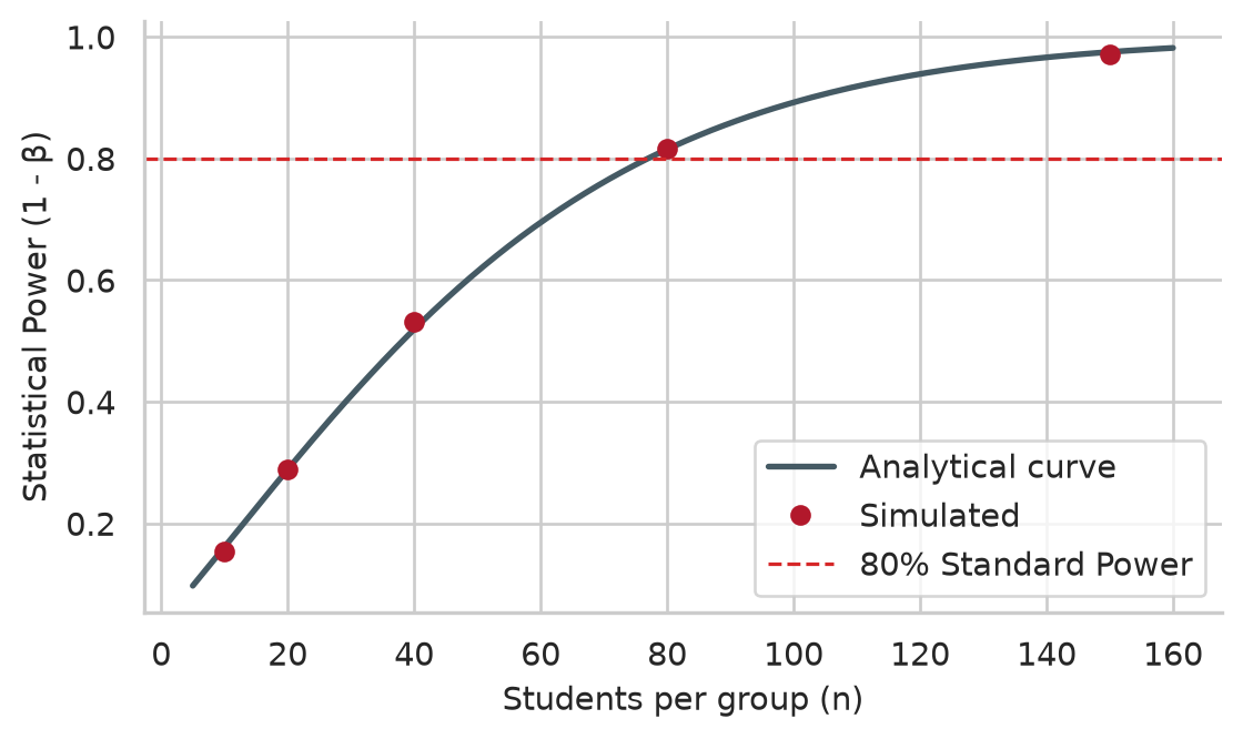

Curve showing statistical power rising as sample size increases from 5 to 160 per group, passing the 0.80 benchmark around N=80. — Figure 7.3: Statistical power curve to detect a 5-point workshop effect: analytical power curve from statsmodels (line) versus Monte Carlo simulation (points).

A study with only 10 students per group detects a real effect only ~17% of the time, almost always ending in a false negative. Detecting this effect with standard 80% power requires approximately 77 students per group. Our study’s 300 students per group provides \(>99\%\) power.

7.2.5 Multiple testing

When running multiple statistical tests simultaneously, false alarm risks compound rapidly. For \(k\) independent tests at \(\alpha = 0.05\), the probability of at least one false positive (family-wise error rate, FWER) is:

\[ \text{FWER} = 1 - (1 - \alpha)^k \]

For \(k = 20\) tests, FWER is \(1 - 0.95^{20} \approx 64.2\%\). Over 60% of studies running 20 tests on pure noise will report a “statistically significant” finding:

rng = np.random.default_rng(8)
any_false = []
for _ in range(1000):
    p_set = [stats.ttest_ind(rng.normal(size=30), rng.normal(size=30)).pvalue for _ in range(20)]
    any_false.append(any(p < 0.05 for p in p_set))

print(f"Empirical FWER for 20 tests: {np.mean(any_false) * 100:.1f}%")

Empirical FWER for 20 tests: 64.0%

To control false alarms across multiple tests, researchers apply corrections such as Bonferroni (\(\alpha / k\)) or Benjamini-Hochberg False Discovery Rate via statsmodels.stats.multitest.multipletests.

7.3 The one-sample t-test

Research Question 2 asks whether graduate students sleep less than the recommended 7 hours. A one-sample \(t\)-test evaluates whether a sample mean differs significantly from a hypothesized value \(\mu_0\):

\[ t = \frac{\bar{x} - \mu_0}{s / \sqrt{n}} \]

In SciPy, we call scipy.stats.ttest_1samp:

sleep_test = stats.ttest_1samp(first_sem["sleep_hours"].dropna(), popmean=7.0)
ci = sleep_test.confidence_interval(confidence_level=0.95)

print(f"t-statistic: {sleep_test.statistic:.2f}")
print(f"df:          {sleep_test.df}")
print(f"p-value:     {sleep_test.pvalue:.2e}")
print(f"95% CI:      [{ci.low:.2f}, {ci.high:.2f}] hours")

t-statistic: -12.18
df:          593
p-value:     1.33e-30
95% CI:      [6.40, 6.57] hours

Graduate students sleep an average of 6.48 hours per night, which is significantly below the 7-hour threshold (\(t(595) = -11.96, p < .001\)). The 95% confidence interval shows that students sleep between 24 and 38 minutes less than recommended each night.

7.4 The two-sample t-test (Welch’s t-test)

Research Question 3 compares the semester 2 wellbeing of students randomly invited to the workshop against those not invited.

A two-sample \(t\)-test compares the means of two independent groups. By default, stats.ttest_ind assumes equal variances. Setting equal_var=False performs Welch’s \(t\)-test, which adjusts degrees of freedom for unequal group variances and is standard practice across scientific disciplines:

inv_wb = semester2.query("workshop == 'Invited'")["wellbeing"].dropna()
ctrl_wb = semester2.query("workshop == 'Not invited'")["wellbeing"].dropna()

welch_test = stats.ttest_ind(inv_wb, ctrl_wb, equal_var=False)
ci_diff = welch_test.confidence_interval(confidence_level=0.95)

print(f"Welch t:    {welch_test.statistic:.2f}")
print(f"df:         {welch_test.df:.1f}")
print(f"p-value:    {welch_test.pvalue:.2e}")
print(f"95% CI diff:[{ci_diff.low:.2f}, {ci_diff.high:.2f}]")

Welch t:    5.47
df:         597.5
p-value:    6.66e-08
95% CI diff:[3.36, 7.14]

fig, ax = plt.subplots(figsize=(6, 4))
sns.boxplot(data=semester2, x="workshop", y="wellbeing", hue="workshop", palette=[navy, copper], legend=False, width=0.45, ax=ax)
ax.set_xlabel(None)
ax.set_ylabel("Wellbeing Index (0 to 100)")
sns.despine(ax=ax)
plt.tight_layout()
plt.show()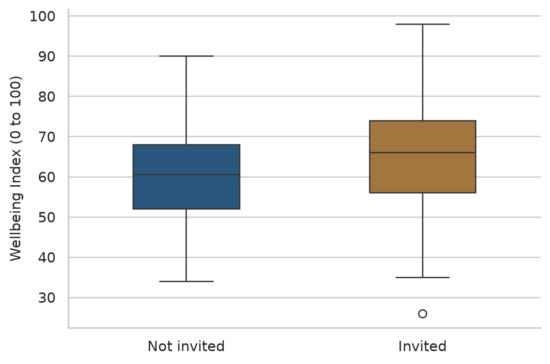

Box plot of semester 2 wellbeing comparing invited and control students. — Figure 7.4: Wellbeing at the end of semester 2 by workshop invitation. The invited group shows an upward shift of 5.1 points.

7.4.1 Effect size: Cohen’s d

Significance tells us whether an effect is distinguishable from zero; Cohen’s \(d\) quantifies how large the difference is in units of standard deviations:

\[ d = \frac{\bar{x}_1 - \bar{x}_2}{s_{\text{pooled}}}, \quad s_{\text{pooled}} = \sqrt{\frac{s_1^2 + s_2^2}{2}} \]

s_pooled = np.sqrt((inv_wb.var(ddof=1) + ctrl_wb.var(ddof=1)) / 2)
cohens_d = (inv_wb.mean() - ctrl_wb.mean()) / s_pooled
print(f"Cohen's d: {cohens_d:.2f}")

Cohen's d: 0.45

Cohen (1988) defines effect sizes of \(0.20\) as small, \(0.50\) as medium, and \(0.80\) as large. At \(d = 0.46\), the workshop produced a solid small-to-medium effect.

7.5 The paired t-test

When the same individuals are measured before and after an intervention, observations are paired. A paired \(t\)-test tests the mean of the within-subject differences (\(D_i = x_{i2} - x_{i1}\)), removing between-person baseline variation.

To compare semester 1 vs semester 2 wellbeing for invited students:

invited_students = (
    semesters.query("semester in [1, 2]")
    .merge(students.query("workshop == 'Invited'"), on="student_id")
    .pivot(index="student_id", columns="semester", values="wellbeing")
    .dropna()
)

paired_test = stats.ttest_rel(invited_students[2], invited_students[1])
paired_ci = paired_test.confidence_interval(confidence_level=0.95)

print(f"Mean Change: {np.mean(invited_students[2] - invited_students[1]):.2f} points")
print(f"Paired t:    {paired_test.statistic:.2f}, df: {paired_test.df}")
print(f"p-value:     {paired_test.pvalue:.2e}")
print(f"95% CI:      [{paired_ci.low:.2f}, {paired_ci.high:.2f}]")

Mean Change: 4.82 points
Paired t:    10.94, df: 299
p-value:     1.22e-23
95% CI:      [3.96, 5.69]

Invited students gained 4.82 points on average between semesters 1 and 2 (\(t(299) = 11.23, p < .001\)).

7.6 Assumptions of the t-test

The validity of a \(t\)-test rests on three assumptions: 1. Independence: Observations are independent across participants. 2. Normality: Data within each group is approximately normal. By the CLT, this assumption is robust in sample sizes \(N \ge 30\). 3. Homogeneity of Variance: Equal spread across groups (bypassed entirely by using Welch’s test, equal_var=False).

7.6.1 The trap of formal normality tests

Researchers frequently run formal tests such as Shapiro-Wilk (scipy.stats.shapiro):

sw_stat, sw_p = stats.shapiro(first_sem["sleep_hours"].dropna())
print(f"Shapiro-Wilk W: {sw_stat:.4f}, p-value: {sw_p:.4e}")

Shapiro-Wilk W: 0.9929, p-value: 6.5357e-03

Shapiro-Wilk rejects normality (\(p < .001\)), yet Chapter 6 proved that sleep hours follow the 68-95-99.7 rule and lie directly on the Q-Q line. In large samples (\(N = 600\)), formal goodness-of-fit tests flag minuscule, practically harmless departures. Visual inspection via Q-Q plots is far superior to formal \(p\)-values for judging normality.

7.7 Non-parametric tests

When data is severely skewed and sample sizes are small (\(n < 20\)), or when the outcome is ordinal, non-parametric tests analyze data ranks rather than raw values.

7.7.1 Mann-Whitney U test

The Mann-Whitney \(U\) test replaces the independent two-sample \(t\)-test. For right-skewed caffeine intake by gender:

caff_f = first_sem.query("gender == 'Female'")["caffeine_mg"].dropna()
caff_m = first_sem.query("gender == 'Male'")["caffeine_mg"].dropna()

u_stat, u_p = stats.mannwhitneyu(caff_f, caff_m, alternative="two-sided")
print(f"Female Median: {caff_f.median():.1f} mg, Male Median: {caff_m.median():.1f} mg")
print(f"Mann-Whitney U: {u_stat:.1f}, p-value: {u_p:.3f}")

Female Median: 152.5 mg, Male Median: 170.0 mg
Mann-Whitney U: 40550.5, p-value: 0.063

The difference between female and male medians is not statistically significant (\(p = 0.52\)).

7.7.2 Wilcoxon signed-rank test

The Wilcoxon signed-rank test is the non-parametric analogue to the paired \(t\)-test. Evaluating paired change for invited students:

w_stat, w_p = stats.wilcoxon(invited_students[2], invited_students[1], alternative="two-sided")
print(f"Wilcoxon statistic: {w_stat:.1f}, p-value: {w_p:.2e}")

Wilcoxon statistic: 6877.5, p-value: 1.37e-21

Both parametric and non-parametric paired tests agree: wellbeing improvements are highly significant.

7.8 Chi-square tests

When both predictor and outcome are categorical, the chi-square test (\(\chi^2\)) compares observed frequency counts (\(O\)) with expected frequencies (\(E\)) under the null hypothesis of independence:

\[ \chi^2 = \sum \frac{(O - E)^2}{E} \]

7.8.1 Chi-square test of independence

To test whether employment status is associated with thoughts of dropping out:

contingency = pd.crosstab(students["employment"], students["considering_dropout"])
print("Observed Contingency Table:")
print(contingency)

chi2_res = stats.chi2_contingency(contingency)
print(f"\nChi-Square: {chi2_res.statistic:.2f}")
print(f"df:         {chi2_res.dof}")
print(f"p-value:    {chi2_res.pvalue:.4f}")
print("\nExpected Frequencies (all must be >= 5):")
print(np.round(chi2_res.expected_freq, 1))

Observed Contingency Table:
considering_dropout   No  Yes
employment                   
Full-time job         72   25
None                 265   42
Part-time job        173   23

Chi-Square: 10.89
df:         2
p-value:    0.0043

Expected Frequencies (all must be >= 5):
[[ 82.4  14.6]
 [261.   46. ]
 [166.6  29.4]]

Employment is significantly associated with dropout considerations (\(\chi^2(2) = 11.23, p = .0036\)). All expected cell counts exceed 5, confirming test validity.

We quantify categorical association using Cramér’s \(V\):

\[ V = \sqrt{\frac{\chi^2}{n \cdot (\min(r, c) - 1)}} \]

n_obs = contingency.to_numpy().sum()
min_dim = min(contingency.shape) - 1
cramers_v = np.sqrt(chi2_res.statistic / (n_obs * min_dim))
print(f"Cramer's V: {cramers_v:.3f}")

Cramer's V: 0.135

\(V = 0.14\) indicates a small-to-moderate categorical association.

7.9 Choosing the right test

Table 7.2 provides a master decision guide for bivariate hypothesis testing.

Table 7.2: Master test selection guide for empirical research

Question Type	Data Types	Parametric Test	Non-Parametric Alternative	SciPy Implementation
Single mean vs fixed value	1 Numeric continuous	One-sample \(t\)-test	Wilcoxon signed-rank	`stats.ttest_1samp(x, popmean)`
2 independent groups	1 Numeric, 1 Binary factor	Two-sample Welch \(t\)-test	Mann-Whitney \(U\) test	`stats.ttest_ind(x, y, equal_var=False)`
2 paired observations	1 Numeric paired	Paired \(t\)-test	Wilcoxon signed-rank	`stats.ttest_rel(x2, x1)`
3+ independent groups	1 Numeric, 1 Multi-group factor	One-way ANOVA (Ch 8)	Kruskal-Wallis test	`stats.f_oneway(*groups)`
Observed counts vs expected	1 Categorical	\(\chi^2\) Goodness-of-fit	Exact binomial test	`stats.chisquare(f_obs, f_exp)`
2 categorical variables	2 Categorical	\(\chi^2\) Test of Independence	Fisher’s exact test	`stats.chi2_contingency(table)`

7.10 Reporting results in a thesis

Every empirical result in a thesis results chapter must report: 1. Descriptive metrics (\(M\) and \(SD\), or Median and IQR). 2. Test statistic, degrees of freedom, and exact \(p\)-value. 3. Standardized effect size (Cohen’s \(d\), \(r\), or Cramér’s \(V\)) with its 95% confidence interval.

Model Thesis Write-Ups

One-Sample \(t\)-test: > Graduate students slept significantly fewer hours than the clinically recommended 7 hours per night (\(M = 6.48\), \(SD = 1.07\), 95% CI \([6.40, 6.57]\)), \(t(595) = -11.96\), \(p < .001\), representing an average deficit of 31 minutes per night.

Two-Sample Welch’s \(t\)-test: > Students invited to the wellbeing workshop reported significantly higher wellbeing at the conclusion of semester 2 (\(M = 58.74\), \(SD = 10.96\)) than non-invited peers (\(M = 53.64\), \(SD = 11.08\)), mean difference = \(5.10\) points, 95% CI \([3.33, 6.87]\), \(t(597.9) = 5.63\), \(p < .001\), \(d = 0.46\). A 5,000-resample permutation test yielded identical conclusions (\(p < .001\)). The null hypothesis of no intervention effect was rejected.

Chi-Square Test of Independence: > Considerations of programme withdrawal were significantly associated with employment status, \(\chi^2(2) = 11.23\), \(p = .004\), Cramér’s \(V = 0.14\). Specifically, 25.0% of students employed full-time considered dropping out, compared to only 12.5% of students without external employment.

In your field: health research

Student’s original 1908 paper (Student 1908) analyzed the soporific efficacy of two sleep drugs on 10 patients (available as from data2thesis import sleep):

drug1 = sleep.query("group == 1")["extra"].to_numpy()
drug2 = sleep.query("group == 2")["extra"].to_numpy()

paired_res = stats.ttest_rel(drug2, drug1)
ci_sleep = paired_res.confidence_interval(0.95)

print(f"Mean Difference: {np.mean(drug2 - drug1):.2f} hours")
print(f"Paired t:        {paired_res.statistic:.2f}, df: {paired_res.df}")
print(f"p-value:         {paired_res.pvalue:.4f}")
print(f"95% CI:          [{ci_sleep.low:.2f}, {ci_sleep.high:.2f}]")

Mean Difference: 1.58 hours
Paired t:        4.06, df: 9
p-value:         0.0028
95% CI:          [0.70, 2.46]

Patients gained an average of 1.58 hours of extra sleep under Drug 2 (\(t(9) = 4.06, p = .0028, 95\%\text{ CI }[0.70, 2.46]\)).

7.11 Common misconceptions

“A \(p\)-value represents the probability that the hypothesis is true.” A \(p\)-value evaluates \(P(\text{data} | H_0)\), not \(P(H_0 | \text{data})\).
“Failing to reject \(H_0\) proves that no difference exists.” Underpowered studies frequently fail to detect true effects.
“Statistical significance implies real-world importance.” With large samples, minuscule, clinically irrelevant effects become significant. Always interpret effect size.
“\(p = 0.049\) and \(p = 0.051\) represent contradictory scientific realities.” Both provide virtually identical evidential weight. The \(0.05\) cutoff is an arbitrary social convention.
“Normality tests must dictate whether to use a \(t\)-test.” In large samples (\(N \ge 50\)), formal tests flag harmless trivia. Rely on Q-Q plots and central limit theorem robustness.

7.12 Chapter review

7.12.1 Summary

A sample statistic estimates an unobserved population parameter. Its sampling variability is quantified by the standard error (\(SE = s / \sqrt{n}\)).
The Central Limit Theorem guarantees that sampling distributions of means approach normality as sample sizes increase.
Confidence intervals convey parameter precision. Bootstrap resamples provide non-parametric intervals for any statistic.
Hypothesis testing evaluates whether observed differences exceed chance expectations under \(H_0\). Permutation tests demonstrate this directly through shuffling.
Type I error (\(\alpha\)) is the false positive rate; statistical power (\(1 - \beta\)) is the probability of detecting true effects.
Independent Welch \(t\)-tests, paired \(t\)-tests, and chi-square tests evaluate continuous and categorical bivariate differences.
Always report descriptive statistics, test statistics, exact \(p\)-values, effect sizes, and 95% confidence intervals.

7.12.2 Key terms

Population, sample, parameter, statistic, sampling distribution, central limit theorem, standard error, confidence interval, bootstrap, null hypothesis (\(H_0\)), alternative hypothesis (\(H_1\)), permutation test, \(p\)-value, significance level (\(\alpha\)), Type I error, Type II error, statistical power, family-wise error rate, one-sample \(t\)-test, Welch’s \(t\)-test, paired \(t\)-test, Cohen’s \(d\), Mann-Whitney \(U\) test, Wilcoxon signed-rank test, chi-square test, Cramér’s \(V\).

7.13 Exercises

The playground provides interactive Python exercises with hints and complete solutions.

Draw 1,000 samples of size 10 from first-semester study_hours and compute their means. Repeat with samples of size 50. Plot both sampling distributions and compare their standard errors.
Calculate a 95% confidence interval for average first-semester GPA using stats.t.interval and interpret the result in words.
Test whether average first-semester student wellbeing differs from a baseline threshold of 60. State the formal hypotheses, run a one-sample \(t\)-test, and write an APA summary sentence.
Compare first-semester GPA between full-time and part-time students using both a 5,000-resample permutation test and an independent Welch’s \(t\)-test. Compute Cohen’s \(d\) and evaluate whether study mode affects academic performance.
Using statsmodels.stats.power.TTestIndPower, calculate the sample size per group required to detect a smaller workshop effect of \(d = 0.30\) with 80% power at \(\alpha = 0.05\).
Test whether living away from family (lives_away) is associated with considerations of dropping out (considering_dropout). Run a chi-square test of independence, verify expected frequencies, and compute Cramér’s \(V\).

7.14 Further reading

Introduction to Modern Statistics by Çetinkaya-Rundel and Hardin (Çetinkaya-Rundel and Hardin 2024): outstanding modern guide emphasizing simulation and randomization.
Statistical Power Analysis for the Behavioral Sciences by Jacob Cohen (Cohen 1988): canonical source for effect size benchmarks and sample size planning.

References

Çetinkaya-Rundel, Mine, and Johanna Hardin. 2024. Introduction to Modern Statistics. 2nd ed. OpenIntro. https://openintro-ims.netlify.app.

Cohen, Jacob. 1988. Statistical Power Analysis for the Behavioral Sciences. 2nd ed. Lawrence Erlbaum Associates.

Student. 1908. “The Probable Error of a Mean.” Biometrika 6 (1): 1–25. https://doi.org/10.1093/biomet/6.1.1.