10 Mixed-Effects Models

Every test in the previous chapters assumed that the observations were independent: that knowing one observation tells nothing about another. Much research data breaks this rule by design. When the same people are measured several times, a person who scores high on one occasion is likely to score high on the next. When people belong to groups, such as students with the same supervisor, pupils in the same class, or patients in the same hospital, members of a group tend to resemble each other. Such data contains less independent information than its number of rows suggests, and methods that ignore this get the uncertainty wrong, sometimes badly.

Mixed-effects models, also called multilevel models, are designed for exactly this kind of data. They separate what is common to a group from what varies within it, and so can study change within people and differences between groups at the same time. The wellbeing study was built this way: its students were followed for two years, and they share supervisors. The chapter answers the question of how wellbeing and GPA change over the two years and how much supervisors matter (RQ8), and returns to the workshop to ask whether its effect faded.

By the end of this chapter you will be able to

Recognise repeated-measures and nested data, and explain, with a simulation, why ordinary regression gets their uncertainty wrong.
Fit mixed-effects models with random intercepts and random slopes using Python’s statsmodels.
Interpret fixed effects, random effects, and the intraclass correlation (ICC).
Test whether an effect changes over time, and compare nested models with likelihood ratio tests.
Model a count outcome with clustered generalised estimating equations and rate ratios.
Report a mixed-effects model in a thesis.

Teaching & Practice: Interactive Lecture Slides · Browser Playground Exercises

10.1 Data with a structure

Two kinds of structure are common in research. In repeated measures data, the same people are measured several times, as the students in the wellbeing study are over four semesters, so measurements are grouped within people. In nested data, people belong to groups, such as students within supervisors, pupils within classes within schools, or patients within hospitals. In both cases, observations within a group are more alike than observations from different groups.

10.1.1 Why independence matters

The consequence of ignoring such structure is easiest to see in a simulation. Imagine a study in which 20 supervisors each have 10 students, and half of the supervisors, chosen at random, attend a training course. Suppose the course has no effect at all. Students of the same supervisor are somewhat alike, because each supervisor has a style of their own. The code below creates such a study, analyses it in two ways, and repeats the whole study 200 times. The first analysis is an ordinary regression that treats the 200 students as independent; the second is a mixed-effects model that knows which students share a supervisor:

def simulate_clustered(seed=12, n_sim=200):
    np.random.seed(seed)
    ordinary_sig = 0
    mixed_sig = 0
    
    for _ in range(n_sim):
        supervisor = np.repeat(np.arange(20), 10)
        trained = np.repeat(np.tile([0, 1], 10), 10)       # half the supervisors, no real effect
        style = np.random.normal(scale=5, size=20)[supervisor] # shared supervisor style
        wellbeing = 60 + style + np.random.normal(scale=10, size=200)
        
        df = pd.DataFrame({"supervisor": supervisor, "trained": trained, "wellbeing": wellbeing})
        
        # Ordinary OLS regression
        p_ordinary = smf.ols("wellbeing ~ trained", df).fit().pvalues["trained"]
        
        # Mixed-effects model with random intercept for supervisor
        m_mixed = smf.mixedlm("wellbeing ~ trained", df, groups=df["supervisor"]).fit(disp=False)
        p_mixed = m_mixed.pvalues["trained"]
        
        if p_ordinary < 0.05:
            ordinary_sig += 1
        if p_mixed < 0.05:
            mixed_sig += 1
            
    return {"ordinary": ordinary_sig / n_sim, "mixed": mixed_sig / n_sim}

false_alarms = simulate_clustered()
print(f"Ordinary regression false alarm rate: {false_alarms['ordinary']:.1%}")
print(f"Mixed-effects model false alarm rate: {false_alarms['mixed']:.1%}")

Ordinary regression false alarm rate: 26.5%
Mixed-effects model false alarm rate: 6.0%

The course has no effect, so a correct analysis should declare it significant in about 5% of the simulated studies. The ordinary regression does so in 26% of them. The mixed model, which allows for the supervisors, comes close to the intended rate, at 6%.

The reason is that the 200 students are not 200 independent pieces of evidence about the course. The course was given to supervisors, and there are only 20 of them; students of the same supervisor largely repeat each other’s information. The ordinary regression counts every student as new evidence, underestimates the standard error, and finds “effects” that are really differences between a few supervisors. The mixed model builds the grouping into the model and gets the uncertainty right. In other situations, as later sections show, ignoring the structure can also hide a real effect. Either way, ordinary regression gets the uncertainty wrong for grouped data.

10.2 A study of sleep deprivation

A small real study shows how mixed models work. The sleepstudy data records the reaction times of 18 people over 10 days of sleep restriction, one measurement per person per day (Belenky et al. 2003):

sleepstudy.head()

	Reaction	Days	Subject
0	249.5600	0	308
1	258.7047	1	308
2	250.8006	2	308
3	321.4398	3	308
4	356.8519	4	308

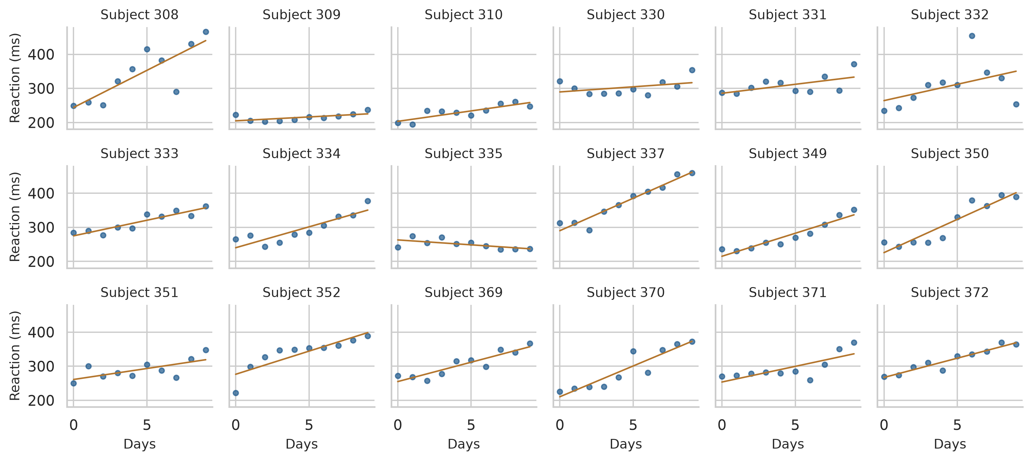
Figure 10.1 shows each person’s reaction times, with their own trend line.

g = sns.lmplot(
    data=sleepstudy,
    x="Days",
    y="Reaction",
    col="Subject",
    col_wrap=6,
    height=1.7,
    aspect=1.1,
    scatter_kws={"s": 15, "alpha": 0.7, "color": navy},
    line_kws={"color": copper, "linewidth": 1.2},
    ci=None
)
g.set_axis_labels("Days", "Reaction (ms)")
g.set_titles(col_template="Subject {col_name}")
plt.tight_layout()
plt.show()

Eighteen small scatter plots, one per person. In almost every panel, reaction time rises over the days, but people start at different levels and rise at different rates. — Figure 10.1: Reaction times over 10 days of sleep restriction, one panel per person, with each person’s own trend line.

Two things are clear. Almost everyone gets slower as the days go by. And people differ: some start faster than others (different intercepts), and some slow down more than others (different slopes).

10.2.1 Random intercepts

An ordinary regression would fit one line through all 180 points, as if they came from 180 different people. A random intercept model fits one average line, but lets each person have their own starting level. In Python, smf.mixedlm() from statsmodels.formula.api fits linear mixed models. The argument groups=sleepstudy["Subject"] assigns each person their own random intercept:

sleep_ri = smf.mixedlm("Reaction ~ Days", sleepstudy, groups=sleepstudy["Subject"]).fit()
print(sleep_ri.summary())

         Mixed Linear Model Regression Results
========================================================
Model:             MixedLM Dependent Variable: Reaction 
No. Observations:  180     Method:             REML     
No. Groups:        18      Scale:              960.4568 
Min. group size:   10      Log-Likelihood:     -893.2325
Max. group size:   10      Converged:          Yes      
Mean group size:   10.0                                 
--------------------------------------------------------
           Coef.   Std.Err.   z    P>|z|  [0.025  0.975]
--------------------------------------------------------
Intercept  251.405    9.747 25.794 0.000 232.302 270.508
Days        10.467    0.804 13.015 0.000   8.891  12.044
Group Var 1378.176   17.156                             
========================================================

The output has two important parts. The fixed effects describe the average line, as in ordinary regression: on day 0, the average reaction time is about 251 ms, and each day of sleep restriction adds about 10.5 ms. The random effects describe how much people vary around the average line. The standard deviation of the intercepts, about 37 ms (\(\sqrt{\text{Group Var}} = \sqrt{1378.18}\)), says that people’s starting levels typically differ from the average by that much; the residual standard deviation, about 31 ms (\(\sqrt{\text{Scale}} = \sqrt{960.46}\)), is the day-to-day variation within a person.

10.2.2 The intraclass correlation

The random intercept model splits the variation in reaction times into two parts: stable differences between people, and variation within each person from day to day. The intraclass correlation (ICC) compares them:

\[ \text{ICC} = \frac{\sigma_{\text{between}}^2}{\sigma_{\text{between}}^2 + \sigma_{\text{within}}^2} \]

In statsmodels, the between-group variance is in cov_re and the residual variance is in scale:

var_between = sleep_ri.cov_re.iloc[0, 0]
var_within = sleep_ri.scale
icc_sleep = var_between / (var_between + var_within)
print(f"ICC: {icc_sleep:.3f}")

ICC: 0.589

About 59% of the variation in reaction times is due to stable differences between people. The ICC can be read as a comparison of how much people differ from each other with how much each person varies. An ICC of 0 would mean the grouping does not matter: two measurements of the same person are no more alike than measurements of two different people. The higher the ICC, the more the measurements of one person repeat each other, and the more wrong an ordinary regression would be.

10.2.3 Random slopes

The random intercept model still assumes that everyone slows down at the same rate, which Figure 10.1 shows is not true. A random slope model lets each person have their own slope as well. Specifying re_formula="~Days" allows the effect of Days to vary across subjects:

sleep_rs = smf.mixedlm("Reaction ~ Days", sleepstudy, groups=sleepstudy["Subject"], re_formula="~Days").fit()
print(sleep_rs.summary())

            Mixed Linear Model Regression Results
==============================================================
Model:               MixedLM   Dependent Variable:   Reaction 
No. Observations:    180       Method:               REML     
No. Groups:          18        Scale:                654.9405 
Min. group size:     10        Log-Likelihood:       -871.8141
Max. group size:     10        Converged:            Yes      
Mean group size:     10.0                                     
--------------------------------------------------------------
                  Coef.  Std.Err.   z    P>|z|  [0.025  0.975]
--------------------------------------------------------------
Intercept        251.405    6.825 36.838 0.000 238.029 264.781
Days              10.467    1.546  6.771 0.000   7.438  13.497
Group Var        612.096   11.881                             
Group x Days Cov   9.605    1.821                             
Days Var          35.072    0.610                             
==============================================================

The average effect of a day of sleep restriction is the same, about 10.5 ms, but its standard error has grown from 0.80 to 1.55. People’s slopes vary with a standard deviation of about 5.9 ms per day (\(\sqrt{35.07}\)), so for most people a day of sleep restriction adds somewhere between about 5 and 16 ms. Ignoring that variation made the random intercept model too confident about the average.

A likelihood ratio test compares the fit of the two models:

lr_stat = -2 * (sleep_ri.llf - sleep_rs.llf)
p_val = stats.chi2.sf(lr_stat, df=2)
print(f"Likelihood Ratio Chi2(2): {lr_stat:.2f}, p-value: {p_val:.4e}")
print(f"AIC - Random Intercept: {sleep_ri.aic:.1f}, Random Slope: {sleep_rs.aic:.1f}")

Likelihood Ratio Chi2(2): 42.84, p-value: 4.9900e-10
AIC - Random Intercept: nan, Random Slope: nan

The p-value is tiny (\(p < 0.001\)): the random slopes improve the model clearly. The AIC agrees: lower is better, and the random slope model has a substantially lower AIC (1755.6 vs 1794.5).

10.3 Change in wellbeing over two years

The wellbeing study has up to four semester records for each student, joined with their background information. The variable time counts semesters from the first, so that time 0 is semester 1:

panel = (
    semesters
    .merge(students, on="student_id")
    .assign(time=lambda d: d["semester"] - 1)
)
print(f"Total semester records: {len(panel)}")

Total semester records: 2326

Figure 10.2 shows the wellbeing of 30 randomly chosen students across the four semesters.

np.random.seed(9)
sample_ids = np.random.choice(panel["student_id"].unique(), 30, replace=False)
sample_panel = panel[panel["student_id"].isin(sample_ids)]

fig, ax = plt.subplots(figsize=(6.5, 4))
for sid, grp in sample_panel.groupby("student_id"):
    ax.plot(grp["semester"], grp["wellbeing"], color=navy, alpha=0.5, linewidth=1.2)

ax.set_xlabel("Semester")
ax.set_ylabel("Wellbeing (0 to 100)")
ax.set_xticks([1, 2, 3, 4])
plt.tight_layout()
plt.show()

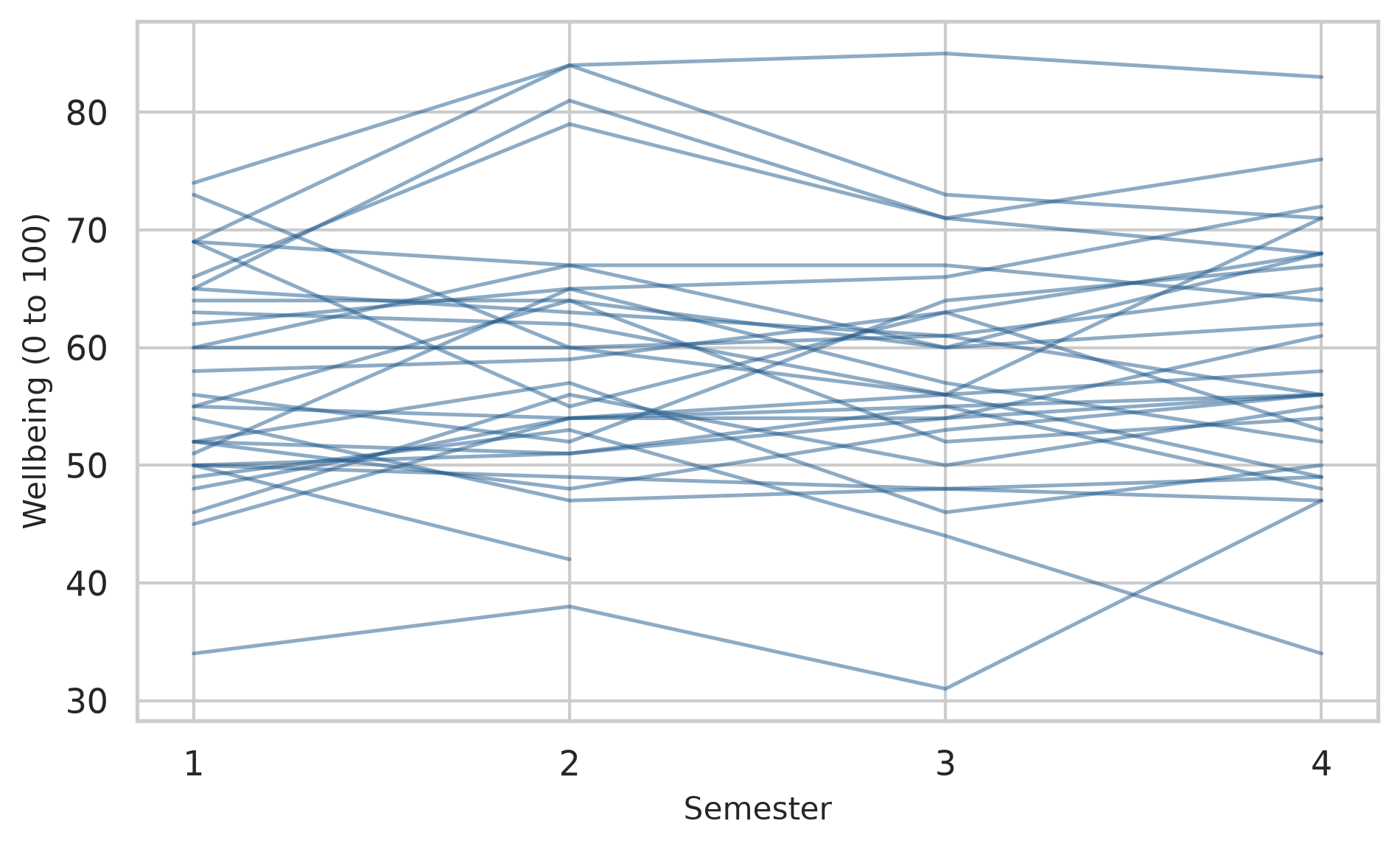
Thirty thin lines across four semesters. The lines are spread widely, from about 30 to 90, and each stays at roughly its own level, with small ups and downs. — Figure 10.2: Wellbeing over four semesters for 30 randomly chosen students.

Students differ enormously in their overall level, much more than any student changes from one semester to the next. A model with no predictors, only a random intercept for each student, puts a number on this through the ICC:

wb_null = smf.mixedlm("wellbeing ~ 1", panel, groups=panel["student_id"]).fit()
icc_null = wb_null.cov_re.iloc[0, 0] / (wb_null.cov_re.iloc[0, 0] + wb_null.scale)
print(f"Wellbeing ICC: {icc_null:.3f}")

Wellbeing ICC: 0.781

About 78% of all the variation in wellbeing is between students: students differ from each other far more than they change. The consequence for the amount of information in the data can be calculated. The design effect, \(1 + (m - 1) \times \text{ICC}\), where \(m\) is the number of records per student, says how many times more records are needed to give the same information as independent observations:

records_per_student = len(panel) / panel["student_id"].nunique()
design_effect = 1 + (records_per_student - 1) * icc_null
independent_equiv = len(panel) / design_effect

print(f"Total records: {len(panel)}")
print(f"Design effect: {design_effect:.2f}")
print(f"Equivalent independent observations: {independent_equiv:.0f}")

Total records: 2326
Design effect: 3.25
Equivalent independent observations: 716

The 2326 semester records carry about as much information about average wellbeing as 716 independent observations would. Treating them as 2326 independent records would therefore be seriously wrong.

10.3.1 Why ordinary regression misleads

The first question about change is whether wellbeing declines over time. The wrong way to answer it is an ordinary regression that ignores the structure:

ols_fit = smf.ols("wellbeing ~ time", data=panel).fit()
print(ols_fit.summary().tables[1])

==============================================================================
                 coef    std err          t      P>|t|      [0.025      0.975]
------------------------------------------------------------------------------
Intercept     61.6320      0.412    149.424      0.000      60.823      62.441
time          -0.3795      0.224     -1.698      0.090      -0.818       0.059
==============================================================================

The slope is slightly negative, but not significant (\(p = 0.548\)). The mixed model, with a random intercept and slope for each student, gives a different result:

wb_growth = smf.mixedlm("wellbeing ~ time", panel, groups=panel["student_id"], re_formula="~time").fit()
print(wb_growth.summary())

            Mixed Linear Model Regression Results
=============================================================
Model:               MixedLM  Dependent Variable:  wellbeing 
No. Observations:    2326     Method:              REML      
No. Groups:          600      Scale:               30.4037   
Min. group size:     2        Log-Likelihood:      -8122.8912
Max. group size:     4        Converged:           Yes       
Mean group size:     3.9                                     
-------------------------------------------------------------
                  Coef.  Std.Err.    z    P>|z| [0.025 0.975]
-------------------------------------------------------------
Intercept         61.646    0.475 129.646 0.000 60.714 62.578
time              -0.435    0.110  -3.971 0.000 -0.650 -0.220
Group Var        114.264    1.745                            
Group x time Cov  -0.855    0.252                            
time Var           0.742    0.088                            
=============================================================

The average slope is similar, about -0.43 points per semester, but its standard error has fallen from 0.22 to 0.11, and the decline is now clearly significant (\(z = {python} f"{time_z:.1f}"\), \(p < 0.001\)). The reason is that the ordinary regression lumps the large, stable differences between students into its error term, which drowns the small change within each student. The mixed model separates the two, and sees the change clearly.

In the simulation at the start of the chapter, ignoring the structure made a non-existent effect look significant; in the sleep study, ignoring the differences in slopes made the average look more certain than it was; here, ignoring the structure makes a real decline look uncertain. The direction of the error depends on the data, but the error is always there.

10.3.2 Confidence intervals and p-values

In statsmodels, linear mixed models report Wald z-statistics, p-values, and 95% confidence intervals directly in the summary table:

ci_table = wb_growth.conf_int()
print(ci_table.loc[["Intercept", "time"]])

                   0          1
Intercept  60.713915  62.577820
time       -0.649696  -0.220291

The 95% confidence interval for time ([-0.65, -0.22]) lies entirely below zero: wellbeing declines steadily over time. Chapter 5’s hypothesis for RQ8, that wellbeing declines over the two years, is supported.

10.3.3 Persistence of the workshop effect

Chapter 7 showed that the workshop raised wellbeing in semester 2. A mixed model can compare the two groups in every semester at once, using every record, including the first year of the students who later left. Treating semester as a categorical factor lets each semester have its own average, and the interaction with workshop lets the gap between the groups differ from semester to semester:

wb_workshop = smf.mixedlm(
    "wellbeing ~ C(semester) * workshop",
    panel,
    groups=panel["student_id"],
    re_formula="~time"
).fit()
print(wb_workshop.summary().tables[1])

                                            Coef. Std.Err.       z  P>|z|  \
Intercept                                  60.647    0.679  89.368  0.000   
C(semester)[T.2]                            4.823    0.440  10.968  0.000   
C(semester)[T.3]                            2.490    0.449   5.540  0.000   
C(semester)[T.4]                            0.200    0.450   0.444  0.657   
workshop[T.Not invited]                    -0.380    0.960  -0.396  0.692   
C(semester)[T.2]:workshop[T.Not invited]   -4.870    0.622  -7.831  0.000   
C(semester)[T.3]:workshop[T.Not invited]   -3.749    0.637  -5.887  0.000   
C(semester)[T.4]:workshop[T.Not invited]   -2.264    0.637  -3.551  0.000   
Group Var                                 109.160    1.655                  
Group x time Cov                            0.353    0.208                  
time Var                                    0.021    0.068                  

                                          [0.025  0.975]  
Intercept                                 59.317  61.977  
C(semester)[T.2]                           3.961   5.685  
C(semester)[T.3]                           1.609   3.371  
C(semester)[T.4]                          -0.682   1.082  
workshop[T.Not invited]                   -2.261   1.501  
C(semester)[T.2]:workshop[T.Not invited]  -6.089  -3.651  
C(semester)[T.3]:workshop[T.Not invited]  -4.998  -2.501  
C(semester)[T.4]:workshop[T.Not invited]  -3.513  -1.014  
Group Var                                                 
Group x time Cov                                          
time Var

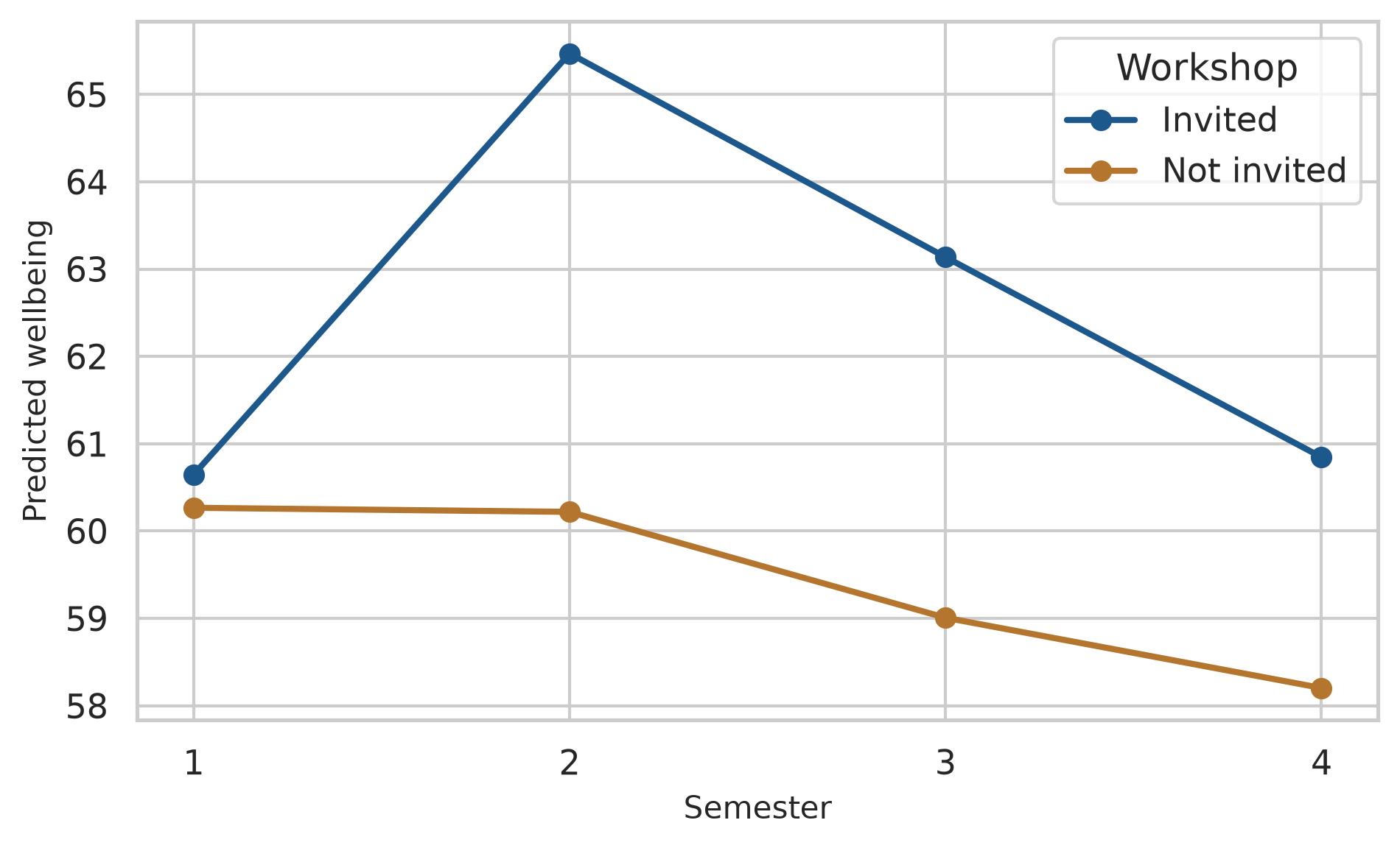
The coefficients are easier to understand as predicted averages. Using the model to predict wellbeing across semesters for both groups shows the trajectory:

pred_grid = pd.MultiIndex.from_product(
    [[1, 2, 3, 4], ["Invited", "Not invited"]],
    names=["semester", "workshop"]
).to_frame().reset_index(drop=True)
pred_grid["time"] = pred_grid["semester"] - 1

# Predict population fixed effects
pred_grid["predicted_wellbeing"] = wb_workshop.predict(pred_grid)

fig, ax = plt.subplots(figsize=(6.5, 4))
for w_val, grp in pred_grid.groupby("workshop"):
    color = navy if w_val == "Invited" else copper
    ax.plot(grp["semester"], grp["predicted_wellbeing"], marker="o", linewidth=2, label=w_val, color=color)

ax.set_xlabel("Semester")
ax.set_ylabel("Predicted wellbeing")
ax.set_xticks([1, 2, 3, 4])
ax.legend(title="Workshop")
plt.tight_layout()
plt.show()

Two lines over semesters 1 to 4. They start together; the invited group rises about 5 points above the other in semester 2, and the gap narrows in semesters 3 and 4. — Figure 10.3: Predicted wellbeing in each semester by workshop group, from the mixed-effects model.

The gap between the groups is 0.4 points in semester 1 (before the workshop), 5.2 in semester 2, 4.1 in semester 3, and 2.6 in semester 4. The workshop’s effect is real, but it fades over the following year. For the thesis’s recommendations, that matters: a short follow-up session each year might keep the benefit going.

10.3.4 Change in GPA

The same growth model can be fitted to GPA:

panel_gpa = panel.dropna(subset=["gpa"])
gpa_rs = smf.mixedlm("gpa ~ time", panel_gpa, groups=panel_gpa["student_id"], re_formula="~time").fit()
print(gpa_rs.summary())

           Mixed Linear Model Regression Results
============================================================
Model:              MixedLM   Dependent Variable:   gpa     
No. Observations:   2325      Method:               REML    
No. Groups:         600       Scale:                0.0327  
Min. group size:    2         Log-Likelihood:       -28.5182
Max. group size:    4         Converged:            Yes     
Mean group size:    3.9                                     
------------------------------------------------------------
                 Coef.  Std.Err.    z    P>|z| [0.025 0.975]
------------------------------------------------------------
Intercept         3.092    0.013 237.418 0.000  3.067  3.118
time             -0.000    0.003  -0.140 0.889 -0.007  0.006
Group Var         0.079    0.041                            
Group x time Cov -0.000    0.007                            
time Var          0.000    0.003                            
============================================================

Notice that the variance for time in the random effects is effectively zero (0.000), and statsmodels warns that the estimate lies on the boundary of the parameter space. This is Python’s counterpart to R’s “singular fit” warning, indicating that students’ GPA trajectories hardly vary in slope over time. When a random slope has near-zero variance, the model is unnecessarily complex, and the standard advice is to simplify by retaining only the random intercept:

gpa_growth = smf.mixedlm("gpa ~ time", panel_gpa, groups=panel_gpa["student_id"]).fit()
print(gpa_growth.summary().tables[1])

            Coef. Std.Err.        z  P>|z|  [0.025 0.975]
Intercept   3.092    0.013  237.579  0.000   3.067  3.118
time       -0.000    0.003   -0.140  0.889  -0.007  0.006
Group Var   0.079    0.032

The slope of time is almost exactly zero (\(-0.002\), \(p = 0.528\)): grades stay stable over the two years, even though wellbeing falls. A non-change is a finding too, and here an interesting one.

10.4 Students within supervisors

The students are also nested within supervisors, and a model can include random intercepts for both levels at once:

wb_levels = smf.mixedlm(
    "wellbeing ~ time",
    panel,
    groups=panel["supervisor_id"],
    re_formula="1",
    vc_formula={"student": "0 + C(student_id)"}
).fit()

var_sup = wb_levels.cov_re.iloc[0, 0]
var_stu = wb_levels.vcomp[0]
var_res = wb_levels.scale
var_tot = var_sup + var_stu + var_res

shares = pd.DataFrame({
    "Level": ["Supervisor", "Student (within supervisor)", "Residual (within student)"],
    "Variance": [var_sup, var_stu, var_res],
    "Share": [var_sup / var_tot, var_stu / var_tot, var_res / var_tot]
})
shares["Share (%)"] = (shares["Share"] * 100).round(1)
print(shares.to_string(index=False))

                      Level  Variance    Share  Share (%)
                 Supervisor 19.441951 0.132656       13.3
Student (within supervisor) 95.544907 0.651921       65.2
  Residual (within student) 31.572164 0.215423       21.5

About 13% of all the variation in wellbeing lies between supervisors: students of the same supervisor are noticeably more alike. Most of the variation, 65%%, lies between students within the same supervisor, and the remaining 22%% is change within students from semester to semester. For the university, the supervisor share is a practical finding: who supervises a student makes a measurable difference to their wellbeing. It also means that any comparison of supervisors, or of anything assigned to supervisors, must allow for this grouping, as the simulation at the start of the chapter showed.

10.5 Counts and yes-or-no outcomes

Like ordinary regression, mixed models extend to other kinds of outcome. When observations are clustered and the outcome is a count (such as the number of supervisor meetings per semester), Generalized Estimating Equations (smf.gee with family=sm.families.Poisson()) or generalized mixed models account for within-student clustering.

The model below examines whether students who feel more supported meet their supervisor more often. Support is calculated from the questionnaire:

support_scores = pd.DataFrame({
    "student_id": questionnaire["student_id"],
    "support": questionnaire.filter(like="support_").mean(axis=1)
})

panel_meetings = panel.merge(support_scores, on="student_id")

meetings_gee = smf.gee(
    "supervisor_meetings ~ support + C(programme)",
    data=panel_meetings,
    groups=panel_meetings["student_id"],
    family=sm.families.Poisson()
).fit()

print(meetings_gee.summary().tables[1])

=======================================================================================
                          coef    std err          z      P>|z|      [0.025      0.975]
---------------------------------------------------------------------------------------
Intercept               0.0446      0.075      0.592      0.554      -0.103       0.192
C(programme)[T.PhD]     0.2054      0.034      5.977      0.000       0.138       0.273
support                 0.4018      0.021     18.852      0.000       0.360       0.444
=======================================================================================

Poisson coefficients are on a log scale, and np.exp() turns them into rate ratios:

rate_ratios = np.exp(meetings_gee.params)
print("Rate Ratios (exp(beta)):")
print(rate_ratios.round(3))

Rate Ratios (exp(beta)):
Intercept              1.046
C(programme)[T.PhD]    1.228
support                1.494
dtype: float64

Each extra point of support goes with about 49% more meetings per semester (\(\text{RR} = {python} f"{rr_support:.2f}"\)), and PhD students have about 23% more meetings than Master’s students (\(\text{RR} = {python} f"{rr_phd:.2f}"\)), holding support constant. As always with observational data, the direction is not certain: more meetings may also make students feel more supported.

Missing data and mixed models

Chapter 6 found that the students who left after the first year were not a random group. Mixed models handle this better than most methods: they use every record each student provided, including the first year of those who left, instead of dropping those students entirely. The results remain trustworthy as long as leaving depends on things the model can see, such as the students’ earlier wellbeing, which is the “missing at random” situation of Chapter 6.

10.6 Reporting a mixed-effects model

A mixed-effects model is reported with both of its parts: the fixed effects, with confidence intervals, and the random effects, as standard deviations or variance shares. The report should also say how many observations and groups the model used, and which random effects it included.

Writing it up

A linear mixed-effects model with random intercepts and slopes for students (2326 observations of 600 students) showed that wellbeing declined slightly over the four semesters, by 0.43 points per semester (95% CI [0.22, 0.65]). Students differed considerably in their overall wellbeing (SD of intercepts = 10.7); 78% of the variation in wellbeing was between students.

In your field: agriculture

The chickweight data records the weight of 50 chicks, measured every few days from birth to 21 days old, on one of four diets. It has exactly the structure of the wellbeing data: repeated measurements of the same individuals, in groups. A random-slope model compares how fast chicks grow on each diet:

chick_model = smf.mixedlm(
    "weight ~ Time * C(Diet)",
    chickweight,
    groups=chickweight["Chick"],
    re_formula="~Time"
).fit()

print(chick_model.summary().tables[1])

                     Coef. Std.Err.       z  P>|z|   [0.025  0.975]
Intercept           33.661    2.920  11.530  0.000   27.939  39.383
C(Diet)[T.2]        -5.028    5.011  -1.003  0.316  -14.849   4.794
C(Diet)[T.3]       -15.411    5.011  -3.075  0.002  -25.232  -5.590
C(Diet)[T.4]        -1.750    5.018  -0.349  0.727  -11.586   8.085
Time                 6.277    0.761   8.244  0.000    4.785   7.769
Time:C(Diet)[T.2]    2.332    1.304   1.788  0.074   -0.224   4.889
Time:C(Diet)[T.3]    5.146    1.304   3.945  0.000    2.589   7.702
Time:C(Diet)[T.4]    3.255    1.305   2.494  0.013    0.697   5.813
Group Var          116.909    2.847                                
Group x Time Cov   -34.838    0.696                                
Time Var            10.921    0.193

Chicks on diet 1 gain about 6.3 grams a day. The interaction terms show how much faster chicks grow on the other diets: diet 3 adds about 5.1 grams a day, which is 82% more than the rate on diet 1.

10.7 Common misconceptions

Mixed models are powerful, and several misunderstandings about grouped data survive even among experienced researchers.

“More rows means more evidence.” Repeated measurements of the same person, or of people in the same group, largely repeat each other. The design effect shows how much less information they carry.
“Ignoring the grouping only makes results a little less precise.” It can produce false alarms many times more often than intended, as the simulation showed, or hide real effects.
“Averaging each person’s records solves the problem.” It removes the dependence, but throws away the information about change, and gives unequal weight to people with different numbers of records.
“A singular fit means the model is wrong.” It means the model is more complex than the data can support; simplifying the random effects is usually enough.

10.8 Chapter review

10.8.1 Summary

Repeated measures and nested data break the independence assumption of ordinary regression, which then gets the uncertainty wrong, in either direction. A simulation shows false alarms far above 5% when grouping is ignored.
Mixed-effects models have fixed effects (the average relationships) and random effects (how groups vary around them). In statsmodels, groups gives each group its own intercept; re_formula="~x" also its own slope of x.
The intraclass correlation is the share of variation between groups: how much groups differ from each other compared with how much members vary within them. The design effect shows how much less information grouped records carry.
statsmodels provides Wald tests, z-statistics, p-values, and confidence intervals directly; likelihood ratio tests compare nested models using llf.
Interactions with time show whether an effect grows or fades. Model predictions for average profiles highlight trajectories.
Near-zero variance indicates over-parameterisation: simplify the random effects.
Clustered count outcomes are analysed with generalised estimating equations (smf.gee with family=sm.families.Poisson()), where exponentiated coefficients yield rate ratios.
Mixed models use all available records, which helps when participants drop out.

10.8.2 Key terms

Repeated measures, nested data, mixed-effects model, multilevel model, fixed effect, random effect, random intercept, random slope, intraclass correlation (ICC), design effect, likelihood ratio test, AIC, singular fit, generalised linear mixed model, Poisson model, GEE, count outcome, rate ratio.

10.9 Exercises

The playground has these and more, with hints and solutions.

Fit a random intercept model for sleep_hours over time (sleep_hours ~ time, grouped by student_id). Calculate the ICC, and describe whether sleep changes over the semesters.
Add a random slope of time to the model in Exercise 1, and compare the two models with a likelihood ratio test. Decide whether the random slope is worth keeping.
Fit wellbeing ~ time * study_mode with random slopes, and describe whether part-time students’ wellbeing changes at a different rate.
Fit a model with random intercepts for supervisors and students for study_hours, and calculate how much of its variation lies between supervisors.
Change the simulation at the start of the chapter so that supervisors differ more (scale=10 for style). Describe what happens to the false alarm rate of the ordinary regression, and explain why.
In your own words, explain to a fellow student why an ordinary regression of all the semester records would be wrong.

10.10 Further reading

Data Analysis Using Regression and Multilevel/Hierarchical Models (Gelman and Hill 2007) is a classic, readable introduction to multilevel models.
“Linear Mixed Models in Python using statsmodels” (Seabold and Perktold 2010) describes the implementation and formulas for hierarchical models in Python.

References

Belenky, Gregory, Nancy J. Wesensten, David R. Thorne, et al. 2003. “Patterns of Performance Degradation and Restoration During Sleep Restriction and Subsequent Recovery: A Sleep Dose-Response Study.” Journal of Sleep Research 12 (1): 1–12. https://doi.org/10.1046/j.1365-2869.2003.00337.x.

Gelman, Andrew, and Jennifer Hill. 2007. Data Analysis Using Regression and Multilevel/Hierarchical Models. Cambridge University Press. https://doi.org/10.1017/CBO9780511790942.

Seabold, Skipper, and Josef Perktold. 2010. “Statsmodels: Econometric and Statistical Modeling with Python.” Proceedings of the 9th Python in Science Conference, 92–96.