import pandas as pd
import numpy as np

clinic = pd.DataFrame({
    'day': range(1, 15),
    'visits': [12, 10, 9, 11, 7, 3, 2,  14, 11, 10, 12, 8, 4, 2]
}).set_index('day')

clinic.head()| visits | |
|---|---|
| day | |
| 1 | 12 |
| 2 | 10 |
| 3 | 9 |
| 4 | 11 |
| 5 | 7 |
Much of the data that organisations keep is recorded over time: patients admitted each day, products sold each month, rainfall each week. Such a sequence of measurements taken at regular intervals is a time series, and it calls for a different way of thinking from the surveys of the previous chapters. The observations are not independent: this week’s value is related to last week’s, and the order of the observations carries information. The patterns are also of a particular kind. A series usually combines a slow trend, a seasonal pattern that repeats over a fixed period, and irregular noise, and understanding a series largely means separating these parts. Finally, the future of a series can never be known exactly, so a forecast is honestly a range of plausible values, not a single number.
This chapter develops these ideas and the methods built on them, using Python’s standard data science and statistical libraries (pandas and statsmodels). The example comes from outside the thesis. The doctors at the university counselling service have heard about Elaf’s wellbeing study and ask her to analyse their records: five years of weekly visit counts, with the service overwhelmed before exams and quiet in the summer, and staffing planned by guesswork. They want to know how many visits to expect next year, week by week. This is an internal analysis, done for the service rather than for publication, and a common situation for anyone who knows some data analysis: being asked to analyse someone else’s data.
Most of this book’s methods assume that observations are independent: one student’s answers tell you nothing about another’s. In a time series the opposite is true. The number of visits this week is closely related to the number last week, and the order of the observations is essential. The methods of this chapter are built around that dependence.
Two weeks of daily visits to a small clinic, starting on a Monday, show how a time series is stored in pandas:
import pandas as pd
import numpy as np
clinic = pd.DataFrame({
'day': range(1, 15),
'visits': [12, 10, 9, 11, 7, 3, 2, 14, 11, 10, 12, 8, 4, 2]
}).set_index('day')
clinic.head()| visits | |
|---|---|
| day | |
| 1 | 12 |
| 2 | 10 |
| 3 | 9 |
| 4 | 11 |
| 5 | 7 |
In pandas, a time series is stored with a dedicated index representing time (either integers representing regular intervals or a DatetimeIndex). The observations are spaced regularly, and operations maintain temporal ordering. There is a clear weekly pattern: busy at the start of the week, quiet at the weekend.
A time series is easiest to understand as a sum of parts. The code below builds an artificial weekly series for three years from three ingredients: a trend that rises slowly, a seasonal pattern that repeats every 52 weeks, and random noise. Figure 16.1 shows each part and their sum.
np.random.seed(4)
weeks = np.arange(1, 157)
trend = 30 + 0.05 * weeks
seasonal = 12 * np.sin(2 * np.pi * weeks / 52)
noise = np.random.normal(0, 3, 156)
series = trend + seasonal + noise

fig, axes = plt.subplots(4, 1, figsize=(7.5, 5.5), sharex=True)
panels = [
    (trend, "Trend"),
    (seasonal, "Seasonal"),
    (noise, "Noise"),
    (series, "Series (Sum)")
]

for ax, (data, title) in zip(axes, panels):
    ax.plot(weeks, data, color="#2f6793", linewidth=1.5)
    ax.set_ylabel(title)
    ax.grid(True, linestyle="--", alpha=0.5)

axes[-1].set_xlabel("Week")
plt.tight_layout()
plt.show()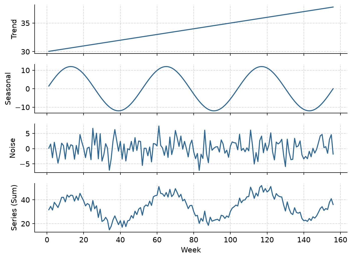
In a real series, only the bottom panel is observed; the parts must be recovered from it. The trend says where the series is heading, the seasonal pattern says what happens at each point in the year, and the noise is what no pattern explains. Forecasting extends the trend and the seasonal pattern into the future. The noise cannot be forecast, and it is the main reason every forecast comes with a range. The decomposition later in this chapter recovers these parts from the counselling data.
The counselling records are loaded via load_counselling_visits(): the date of the Monday of each week, and the number of visits that week.
counselling_visits = dt.load_counselling_visits()
counselling_visits['week_start'] = pd.to_datetime(counselling_visits['week_start'])
print(counselling_visits.head())
print(f"Date range: {counselling_visits['week_start'].min().date()} to {counselling_visits['week_start'].max().date()}")
print(f"Total weeks: {len(counselling_visits)}")
week_start visits
0 2020-09-07 32
1 2020-09-14 28
2 2020-09-21 24
3 2020-09-28 37
4 2020-10-05 32
Date range: 2020-09-07 to 2025-08-25
Total weeks: 260The data covers five academic years, from September 2020 to August 2025, 260 weeks in all. Setting the datetime column as the index gives a clean time series structure:
visits = counselling_visits.set_index('week_start').sort_index()
visits.head()| visits | |
|---|---|
| week_start | |
| 2020-09-07 | 32 |
| 2020-09-14 | 28 |
| 2020-09-21 | 24 |
| 2020-09-28 | 37 |
| 2020-10-05 | 32 |
The first step with any time series is to draw a time plot:
plt.figure(figsize=(8, 3.8))
plt.plot(visits.index, visits['visits'], color="#2f6793", linewidth=1.5)
plt.ylabel("Visits per week")
plt.grid(True, linestyle="--", alpha=0.5)
plt.tight_layout()
plt.show()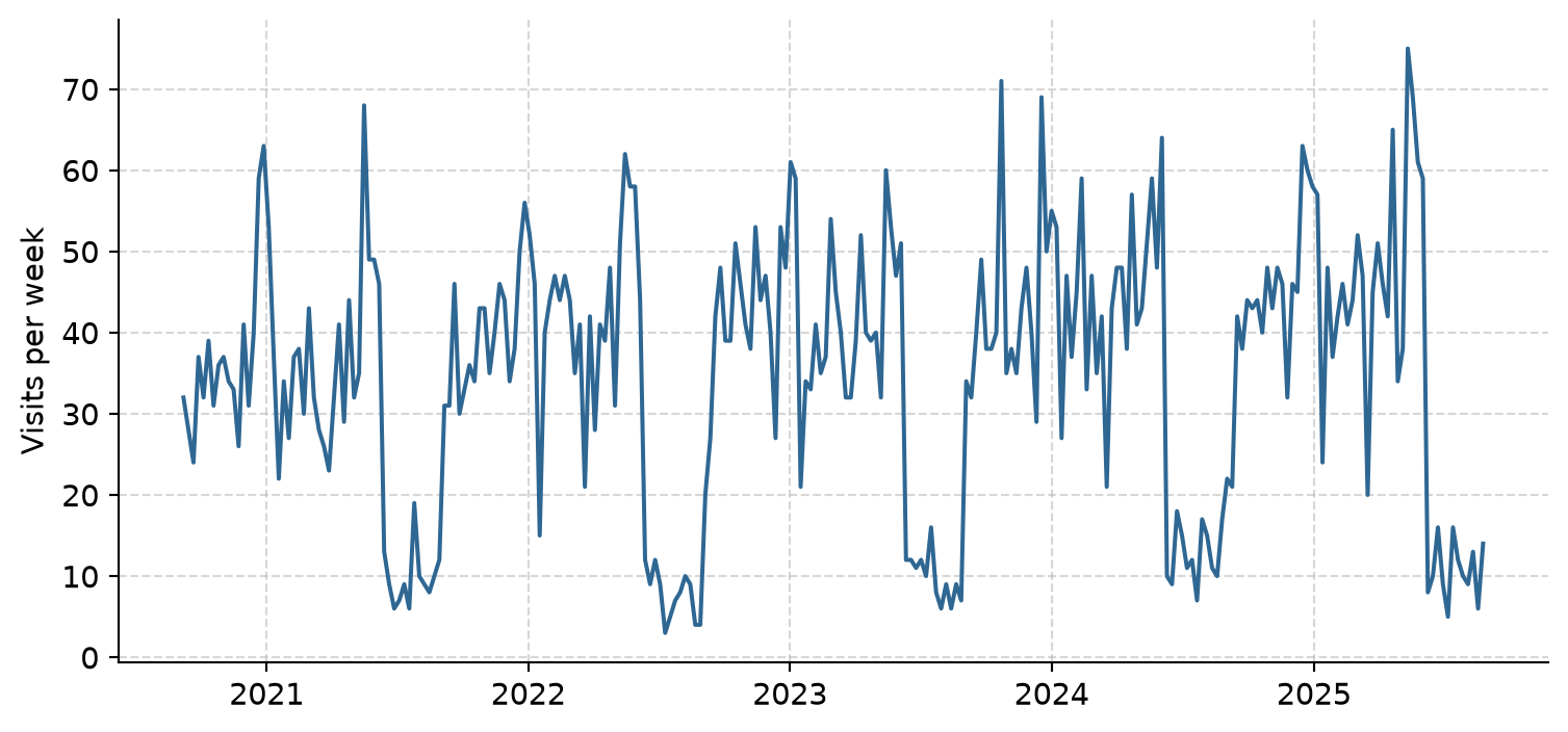
Figure 16.2 shows the parts of a pattern described above, and one feature the doctors did not mention. There is a seasonal pattern that repeats every academic year: peaks before and during the two exam periods, dips during the breaks, and very few visits in the summer, when the service is reduced. There is a gentle upward trend, each year a little busier than the last, and there is noise, week-to-week variation that follows no pattern. Finally, there is one unusual week, in the autumn of 2023, far busier than the weeks around it.
A seasonal plot puts the years on top of each other, so the seasonal pattern and the differences between years are easier to see. The academic year starts in September, so the weeks are numbered from 1 to 52 across each academic year:
visits_seasonal = visits.copy()
visits_seasonal['year_idx'] = np.arange(len(visits_seasonal)) // 52
visits_seasonal['week_of_year'] = (np.arange(len(visits_seasonal)) % 52) + 1
visits_seasonal['academic_year'] = visits_seasonal['year_idx'].apply(lambda i: f"20{20+i}/{21+i}")

plt.figure(figsize=(7.5, 4))
colors = plt.cm.viridis(np.linspace(0.1, 0.9, 5))

for (acad_year, group), col in zip(visits_seasonal.groupby('academic_year'), colors):
    plt.plot(group['week_of_year'], group['visits'], label=acad_year, color=col, linewidth=1.8)

plt.xlabel("Week of the academic year")
plt.ylabel("Visits per week")
plt.legend(title="Academic year")
plt.grid(True, linestyle="--", alpha=0.5)
plt.tight_layout()
plt.show()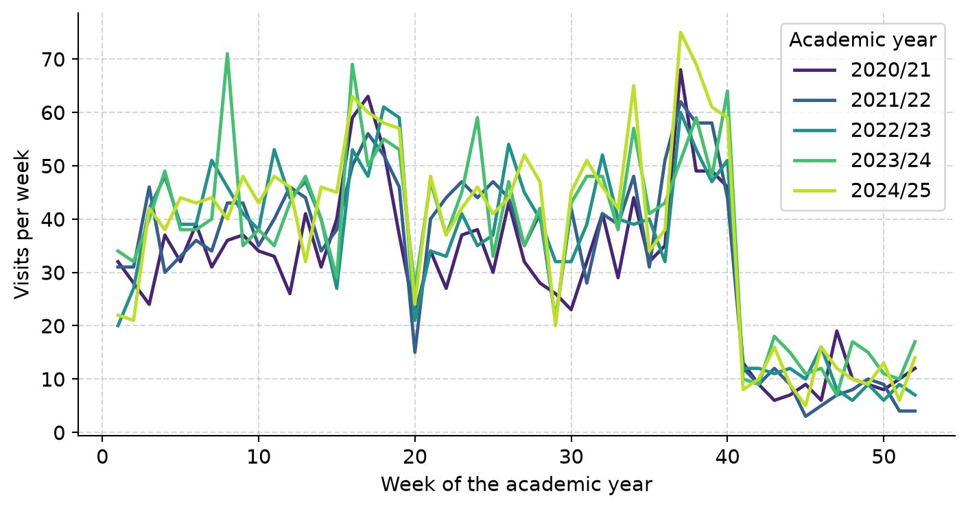
Every year has the same shape, and later years lie slightly above earlier ones. The period of the seasonal pattern is 52 weeks.
Dependence over time can be seen directly by plotting each week’s visits against the visits one week earlier, as in Figure 16.4.
plt.figure(figsize=(5, 4))
plt.scatter(visits['visits'].shift(1), visits['visits'], color="#2f6793", alpha=0.6, edgecolors="none")
plt.xlabel("Visits in the previous week (lag 1)")
plt.ylabel("Visits this week")
plt.grid(True, linestyle="--", alpha=0.5)
plt.tight_layout()
plt.show()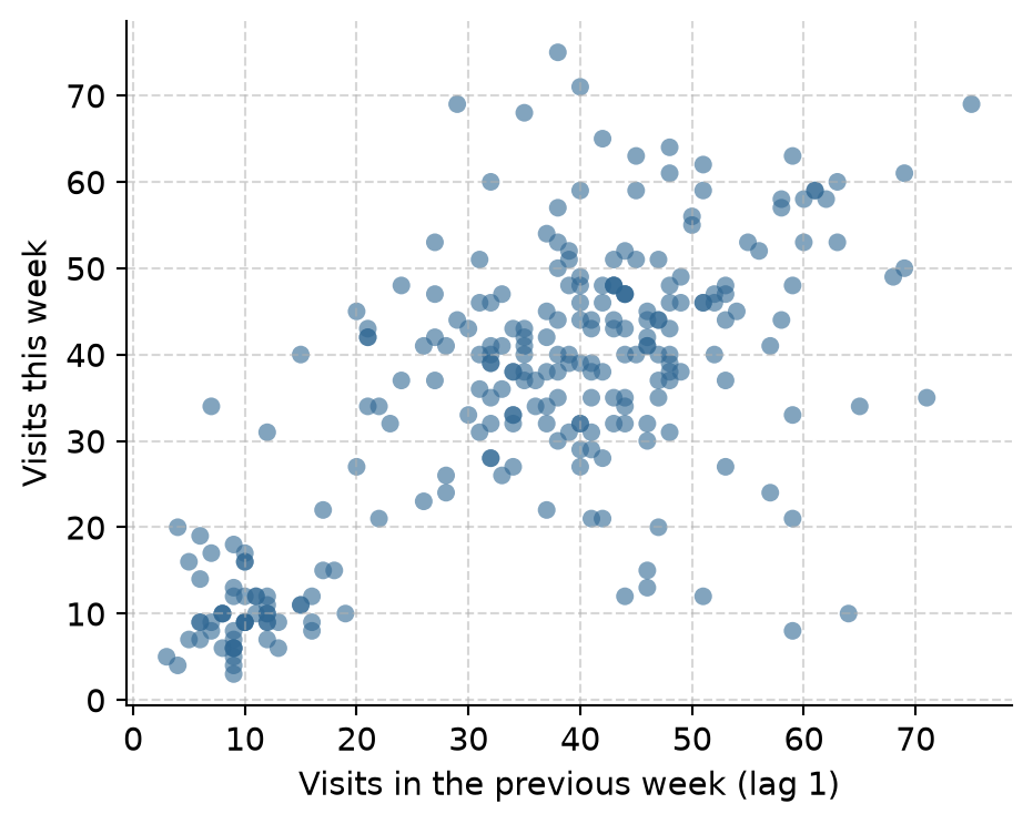
The points rise from left to right: knowing last week’s visits says a good deal about this week’s. The autocorrelation at lag \(k\) puts a number on this relationship: it is the correlation between the series and itself \(k\) steps earlier, between each week and the week before (lag 1), two weeks before (lag 2), and so on. In Python, acf() from statsmodels.tsa.stattools calculates it:
from statsmodels.tsa.stattools import acf

visits_acf = acf(visits['visits'], nlags=60)
print(f"Lag 1 autocorrelation:  {visits_acf[1]:.2f}")
print(f"Lag 26 autocorrelation: {visits_acf[26]:.2f}")
print(f"Lag 52 autocorrelation: {visits_acf[52]:.2f}")
Lag 1 autocorrelation: 0.69
Lag 26 autocorrelation: -0.24
Lag 52 autocorrelation: 0.68The autocorrelation is 0.69 at lag 1, as the scatter plot suggested, and 0.68 at lag 52: a week tends to be like the same week a year earlier. At lag 26 it is negative (−0.24): half a year apart, a busy term week is often matched with a quiet summer week. Figure 16.5 shows all the lags. Strong autocorrelation at the seasonal lag is the signature of seasonality; if a series had no autocorrelation at all, there would be nothing to forecast beyond its average.
from statsmodels.graphics.tsaplots import plot_acf

fig, ax = plt.subplots(figsize=(7, 3.2))
plot_acf(visits['visits'], lags=60, ax=ax, color="#2f6793", vlines_kwargs={"colors": "#2f6793"})
ax.set_xlabel("Lag (weeks)")
ax.set_ylabel("Autocorrelation")
ax.grid(True, linestyle="--", alpha=0.5)
plt.tight_layout()
plt.show()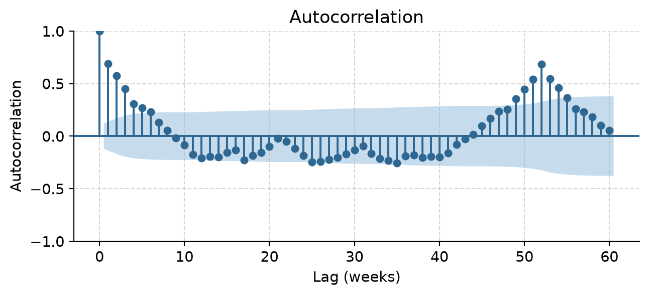
Decomposition recovers the parts of a pattern from an observed series: a smooth trend, a repeating seasonal component, and the remainder, what is left over, which corresponds to the noise of Figure 16.1. STL (seasonal and trend decomposition using loess) is a flexible, widely used method available in statsmodels.tsa.seasonal.STL. Setting period=52 specifies the annual cycle, and robust=True prevents extreme weeks from distorting the trend:
from statsmodels.tsa.seasonal import STL

stl = STL(visits['visits'], period=52, robust=True)
visits_stl = stl.fit()
fig, (ax1, ax2, ax3, ax4) = plt.subplots(4, 1, figsize=(8, 6), sharex=True)
ax1.plot(visits.index, visits['visits'], color="#2f6793", linewidth=1.2)
ax1.set_ylabel("Data")
ax2.plot(visits.index, visits_stl.trend, color="#2f6793", linewidth=1.2)
ax2.set_ylabel("Trend")
ax3.plot(visits.index, visits_stl.seasonal, color="#2f6793", linewidth=1.2)
ax3.set_ylabel("Seasonal")
ax4.plot(visits.index, visits_stl.resid, color="#2f6793", linewidth=1.2)
ax4.set_ylabel("Remainder")
for ax in (ax1, ax2, ax3, ax4):
ax.grid(True, linestyle="--", alpha=0.5)
plt.tight_layout()
plt.show()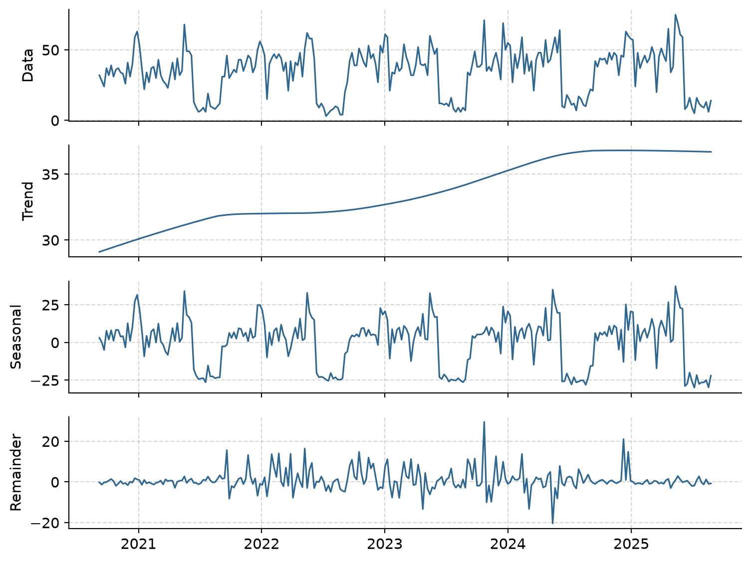
In Figure 16.6 the series is the sum of the three components below it, just as in the artificial example. The trend rises from about 35 to about 41 visits a week, levelling off in the last year; the seasonal component repeats the academic year; and the remainder is mostly small noise. The largest remainder is the unusual week:
decomp_df = pd.DataFrame({
    'week': visits.index,
    'visits': visits['visits'].values,
    'trend': visits_stl.trend.values,
    'seasonal': visits_stl.seasonal.values,
    'remainder': visits_stl.resid.values
})

top_remainders = decomp_df.iloc[decomp_df['remainder'].abs().argsort()[::-1][:3]]
print(top_remainders[['week', 'visits', 'trend', 'seasonal', 'remainder']].round(1))
week visits trend seasonal remainder
163 2023-10-23 71 34.7 6.8 29.5
222 2024-12-09 45 36.8 -12.9 21.1
192 2024-05-13 51 36.3 35.1 -20.4In the week of 23 October 2023, there were 71 visits, about 30 more than trend and season would predict. When asked, the doctors remember at once: it was the university’s mental health awareness week, with posters everywhere encouraging students to seek help. The remainder is where such events show up. It is a real week, not an error, so it is kept, and the robust decomposition makes sure it does not distort the forecasts.
Notice also that the seasonal swings grow slightly as the trend rises: the peaks get higher and the summer lows stay low. When the seasonal pattern grows in proportion to the level of the series, it is standard practice to model the logarithm of the series, on which the swings become additive and stable.
Every forecasting method should be compared with simple benchmark methods, just as every predictive model in Chapters 11 to 13 was compared with a baseline. The three most common are:
For the clinic example, with its weekly cycle of 7 days:
y_clinic = clinic['visits'].values

mean_fc   = np.repeat(np.mean(y_clinic), 7)
naive_fc  = np.repeat(y_clinic[-1], 7)
snaive_fc = y_clinic[-7:]

pd.DataFrame({
    'Day': range(15, 22),
    'Mean': mean_fc.round(1),
    'Naive': naive_fc,
    'Seasonal_Naive': snaive_fc
}).set_index('Day')| Mean | Naive | Seasonal_Naive | |
|---|---|---|---|
| Day | |||
| 15 | 8.2 | 2 | 14 |
| 16 | 8.2 | 2 | 11 |
| 17 | 8.2 | 2 | 10 |
| 18 | 8.2 | 2 | 12 |
| 19 | 8.2 | 2 | 8 |
| 20 | 8.2 | 2 | 4 |
| 21 | 8.2 | 2 | 2 |
The mean method forecasts 8.4 visits every day; the naive method repeats the last value (a quiet Sunday of 2 visits) for the whole week; and the seasonal naive method repeats last week’s pattern, which for this series is clearly the most sensible.
Two families of models go beyond the benchmarks:
Both work best with short seasonal periods, such as 4 quarters, 7 days, or 12 months. A 52-week season is long, so two strategies are common: 1. Decompose first (STL + ETS): decompose the log series with STL, forecast the seasonally adjusted series with ETS, and add the seasonal component back. 2. Fourier terms with ARIMA: model the 52-week seasonal wave using pairs of sine and cosine terms (Fourier series) as external regressors.
As in machine learning, forecasts must be judged on data the model has not seen. For time series, the test data must come after the training data, because a forecast can only use the past. The models are trained on the first four academic years (208 weeks) and tested on the fifth (52 weeks):
train = visits[visits.index < '2024-09-01'].copy()
test  = visits[visits.index >= '2024-09-01'].copy()

y_train = train['visits'].values
y_test  = test['visits'].values
h = len(test)

# Benchmarks
fc_mean   = np.repeat(np.mean(y_train), h)
fc_naive  = np.repeat(y_train[-1], h)
fc_snaive = y_train[-52:]

# Model 1: STL + ETS
from statsmodels.tsa.api import Holt

log_y_train = np.log(y_train)
stl_tr = STL(log_y_train, period=52, robust=True).fit()
sa_tr = log_y_train - stl_tr.seasonal

ets_fit = Holt(sa_tr, initialization_method='estimated').fit()
fc_sa = ets_fit.forecast(h)
fc_stl_ets = np.exp(fc_sa + stl_tr.seasonal[-52:])

# Model 2: Fourier + ARIMA
from statsmodels.tsa.arima.model import ARIMA

K = 6
t_tr = np.arange(len(y_train))
t_te = np.arange(len(y_train), len(y_train) + h)
X_tr = np.column_stack([fn(2 * np.pi * k * t_tr / 52) for k in range(1, K + 1) for fn in (np.sin, np.cos)])
X_te = np.column_stack([fn(2 * np.pi * k * t_te / 52) for k in range(1, K + 1) for fn in (np.sin, np.cos)])

arima_fit = ARIMA(log_y_train, order=(1, 0, 0), exog=X_tr).fit()
fc_fourier = np.exp(arima_fit.forecast(h, exog=X_te))
Each model forecasts the 52 weeks of the test year, and we evaluate their accuracy using RMSE and MAE:
from sklearn.metrics import mean_squared_error, mean_absolute_error

models = {
    'Mean': fc_mean,
    'Naive': fc_naive,
    'Seasonal naive': fc_snaive,
    'STL + ETS': fc_stl_ets,
    'Fourier + ARIMA': fc_fourier
}

acc_table = []
for name, preds in models.items():
    rmse = np.sqrt(mean_squared_error(y_test, preds))
    mae = mean_absolute_error(y_test, preds)
    acc_table.append({'Model': name, 'RMSE': round(rmse, 2), 'MAE': round(mae, 2)})

pd.DataFrame(acc_table).sort_values('RMSE').reset_index(drop=True)| Model | RMSE | MAE | |
|---|---|---|---|
| 0 | Seasonal naive | 9.16 | 6.96 |
| 1 | STL + ETS | 9.35 | 6.81 |
| 2 | Fourier + ARIMA | 11.37 | 8.93 |
| 3 | Mean | 18.67 | 16.33 |
| 4 | Naive | 27.54 | 23.50 |
The STL and ETS model is best: its forecasts are off by 6.8 visits a week on average (MAE), against 7.0 for the seasonal naive benchmark, which simply repeats the previous year. The mean and naive methods, which ignore the seasonal pattern, are far worse. The Fourier model does worse than the seasonal naive benchmark: the counselling service’s pattern has sharp steps (the summer drop happens from one week to the next), and smooth waves struggle to follow them. Figure 16.7 compares the two best models with the actual visits.
plt.figure(figsize=(8, 3.8))
plt.plot(test.index, y_test, color="black", linewidth=2, label="Actual visits")
plt.plot(test.index, fc_stl_ets, color="#2f6793", linewidth=1.8, label="STL + ETS")
plt.plot(test.index, fc_snaive, color="#d95f02", linestyle="--", linewidth=1.5, label="Seasonal naive")

plt.ylabel("Visits per week")
plt.legend()
plt.grid(True, linestyle="--", alpha=0.5)
plt.tight_layout()
plt.show()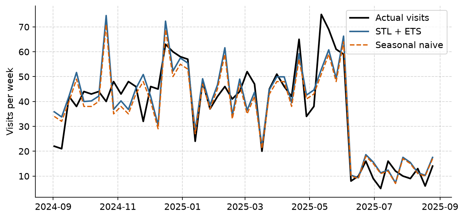
The seasonal naive forecast copies last year’s noise along with its pattern: it even repeats the awareness week of October 2023 as a spike in October 2024. The STL and ETS model smooths the noise away and adds the trend, so its forecasts are both smoother and closer.
With the model chosen, it is refitted on all five years of data (260 weeks), so the forecasts use the most recent information, and the next 52 weeks are forecast:
y_all = visits['visits'].values
log_y_all = np.log(y_all)

stl_full = STL(log_y_all, period=52, robust=True).fit()
sa_full = log_y_all - stl_full.seasonal

ets_full = Holt(sa_full, initialization_method='estimated').fit()
fc_sa_next = ets_full.forecast(52)
fc_log_next = fc_sa_next + stl_full.seasonal[-52:]
fc_next_year = np.exp(fc_log_next)

next_dates = pd.date_range(start=visits.index[-1] + pd.Timedelta(weeks=1), periods=52, freq='W-MON')
resid = stl_full.resid
sigma = np.std(resid)
lower_80 = np.exp(fc_log_next - 1.28 * sigma)
upper_80 = np.exp(fc_log_next + 1.28 * sigma)
lower_95 = np.exp(fc_log_next - 1.96 * sigma)
upper_95 = np.exp(fc_log_next + 1.96 * sigma)
recent = visits[visits.index >= '2023-09-01']
plt.figure(figsize=(8, 3.8))
plt.plot(recent.index, recent['visits'], color="black", label="Observed", linewidth=1.5)
plt.plot(next_dates, fc_next_year, color="#2f6793", label="Forecast", linewidth=2)
plt.fill_between(next_dates, lower_95, upper_95, color="#2f6793", alpha=0.15, label="95% Interval")
plt.fill_between(next_dates, lower_80, upper_80, color="#2f6793", alpha=0.25, label="80% Interval")
plt.ylabel("Visits per week")
plt.legend(loc="upper left")
plt.grid(True, linestyle="--", alpha=0.5)
plt.tight_layout()
plt.show()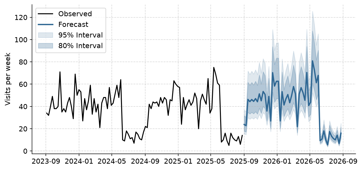
A forecast is never a single number. The shaded bands in Figure 16.8 are prediction intervals: the ranges within which the actual visits are expected to fall with 80% and 95% probability.
next_df = pd.DataFrame({
    'Week': next_dates,
    'Forecast': fc_next_year.round(1),
    'Lower 95%': lower_95.round(1),
    'Upper 95%': upper_95.round(1)
}).set_index('Week')

next_df.head(4)| Forecast | Lower 95% | Upper 95% | |
|---|---|---|---|
| Week | |||
| 2025-09-01 | 23.8 | 15.4 | 36.9 |
| 2025-09-08 | 22.7 | 14.7 | 35.3 |
| 2025-09-15 | 46.3 | 29.9 | 71.8 |
| 2025-09-22 | 44.3 | 28.6 | 68.7 |
In the first week of the new year, about 24 visits are expected, but anything from about 17 to 33 would not be surprising. The doctors also asked for the year as a whole. Adding up weekly forecasts gives the expected total, but not its uncertainty, because weeks do not vary independently. We estimate this by simulation: producing 1,000 possible futures from the model by sampling the empirical residuals:
np.random.seed(2026)
sim_totals = []
for _ in range(1000):
    sim_noise = np.random.choice(resid, size=52, replace=True)
    sim_path = np.exp(fc_log_next + sim_noise)
    sim_totals.append(np.sum(sim_path))

q = np.quantile(sim_totals, [0.025, 0.5, 0.975]).round()
last_year_total = np.sum(test['visits'])

print(f"Predicted total visits for 2025/26: {int(q[1]):,}")
print(f"95% Prediction Interval:             {int(q[0]):,} to {int(q[2]):,}")
print(f"Actual total visits in 2024/25:      {int(last_year_total):,}")
Predicted total visits for 2025/26: 2,177
95% Prediction Interval: 2,050 to 2,464
Actual total visits in 2024/25: 1,954The report to the service therefore says: about 2,177 visits are expected in 2025/26 (95% interval 2,050 to 2,464), compared with 2,056 in 2024/25; the busiest weeks will again be just before and during the two exam periods, when they should plan the most staff; and an awareness campaign can raise demand sharply for a week, so extra capacity should be planned for any such event.
Every forecast in this chapter assumes that the patterns of the last five years continue. A change the data cannot know about, such as a new online booking system, a change in the exam calendar, or a crisis like the COVID-19 pandemic, can make any forecast wrong. Report forecasts with their intervals, say what they assume, and update them as new data arrives.
Time series have their own traps, most of them versions of forgetting that time has an order.
Time series, datetime index, time plot, trend, seasonality, seasonal period, seasonal plot, autocorrelation, lag, decomposition, STL, remainder, seasonally adjusted series, benchmark forecast, mean method, naive method, seasonal naive method, exponential smoothing (ETS), ARIMA, SARIMAX, Fourier terms, forecast horizon, prediction interval, simulation.
The playground has these and more, with hints and solutions.
clinic after adding a steady increase of one visit a day.sa = visits - stl.seasonal), and describe what it shows that the original series hides.