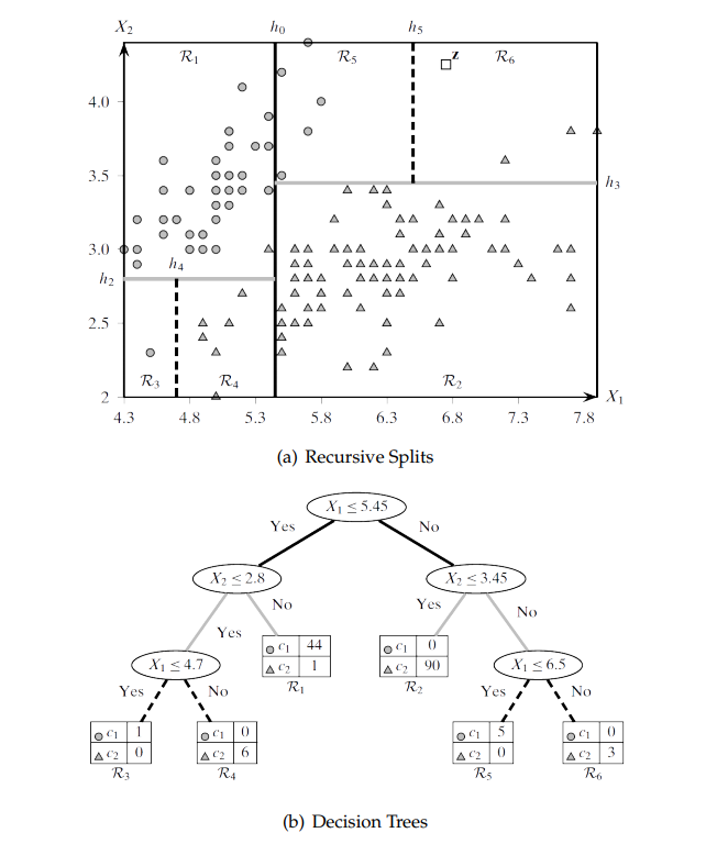
As described by Zaki et al. 1, Decision Tree is a classification model which recursively partitions the data space into two parts. The split can be considered as a hyperplane parallel to one axis of the data space. The process repeats by dividing each new part into two smaller parts, and this process continues until each sub-part mostly contains items of only one of the target classes. The final result of this partitioning process can be represented by a tree, where each node is a decision concerning which part an item belongs to, and the leaves represent one of the target classes.
As an example of the decision tree partitioning, consider the iris data set with 150 entries of three classes. The items are displayed in Figure below, which plots their sepal length and width as X, Y axes. The partitioning process created six different regions, which are divided by lines instead of hyperplains, as in two-dimensional data space the hyperplanes can only have one dimension. Multiple regions might represent one of the targeted classes. The tree representation of the iris data space partition is shown in Figure \ref{fig:Recurcive2Decision2}.

C4.5 might be one of the most famous decision tree algorithms for classification 2. C4.5 is build on ID3, both of which were introduced by Quinlan 3. This algorithm relies on information gained to create its tree for classification. In this algorithm attributes with higher normalised information gain are used for decide the splits in the data. The the next highest attribute is used for subpartitioning the data recursively 3.
This algorithm is superseded by a new version C5.0, which is more efficient as it uses less memory and functions more efficiently and effectively, generating a smaller and more concise decision tree, while it is more general as it can classify more data types than its predecessor. It also incorporates boosting, which means multiple classifier trees can be generated and they will vote for predicting items’ classes. Boosting is a bootstrap aggregate (bagging) mechanism which may improve the stability and accuracy of the final result of the classifier 2. The last aspect of the algorithm is similar to what is provided by Random Forest algorithm, which creates many decision trees from random subsets of the training data 4.
C4.5 has two drawbacks 5, the first of which is overfitting, which might be solved by pruning the decision tree to be more general. Two types of pruning can be done on the tree pre-pruning and post-pruning. Pre-pruning is the operation of preventing particular branches from growing when information becomes unreliable. Post-pruning is the operation of cutting branches of a fully grown tree to remove unreliable parts. The second drawback originates from the very nature of the algorithm by selecting attributes with the highest information gain value. This process will become bias to the attributes with a large number of values.
Conditional Inference Tree (Ctree) was introduced by Hothorn et al. 5 to overcome the attribute bias of the information gain based algorithms. This algorithm uses significance to select covariants of attributes. The significance is determined through P-value which is derived from ANOVA F-statistics. During the training phase, all data permutations will be tested to calculate the p-value.
Reference
-
Zaki, M. J. and Meira, M. J. (2014) Data Mining and Analysis: Fundamental Concepts and Algorithms, Cambridge University Press. New York: Cambridge University Press. ↩
-
Wu, X. et al. (2008) ‘Top 10 algorithms in data mining’, Knowledge and Information Systems, 14(1), pp. 1–37. doi: 10.1007/s10115-007-0114-2. ↩ ↩2
-
Quinlan, J. R. (2014) C4.5: programs for machine learning. Elsevier (C4.5 - programs for machine learning / J. Ross Quinlan). ↩ ↩2
-
Breiman, L. (2001) ‘Random forest’, Machine learning, 45(1), pp. 5–32. doi: 10.1017/CBO9781107415324.004. ↩
-
Hothorn, T., Hornik, K. and Zeileis, A. (2006) ‘Unbiased Recursive Partitioning: A Conditional Inference Framework’, Journal of Computational and Graphical Statistics, 15(3), pp. 651–674. ↩ ↩2