Most statistics books are organised around methods. I organised From Data to Thesis around a person. The book follows Elaf, a new Master’s student in Educational Psychology who noticed how tired her fellow students were, and turned that observation into a thesis about sleep, stress, supervisor support, and wellbeing. The data are a simulated study of 600 graduate students followed over four semesters, and the book says plainly that they are synthetic and not evidence about real students.
That choice shapes the chapter titles. They are not “Chapter 7: The t-distribution”. They are stages of a research project. This post goes through the nineteen chapters in order and says what each one covers beyond the technique. The full book is at polla.dev/data2thesis_r.
Part 1: Foundations (Chapters 1–4)
1. Getting Started with R. The first section is called Research written in code, and it makes the case for the whole book: an analysis typed into a script can be rerun, inspected, and corrected, while one made by clicking cannot. The chapter ends with RStudio Projects, which also helps keep a thesis folder organised from the start.
2. Data Structures in R. The title sounds technical, but the sections begin with Data as measurement. Before any code, the reader is asked what a number represents. Later sections include A codebook and SPSS and Excel equivalents, which meet researchers where they come from, and Error messages, which treats red text as information and not failure.
3. Data Manipulation. The survey export has 615 rows although there are only 600 students, and 64 columns because four semesters are squeezed into one row per student. Cleaning means removing 3 test responses and 12 duplicates, recoding the missing-answer codes 99 and −9, setting 4 impossible values (such as 26 hours of sleep a night) to missing, and reversing a reverse-worded item before computing scale scores. One point from this chapter: every filter is a decision about the sample, and it should be reported.
4. Data Visualization. The sections How people read graphs, Honest graphs, and Common misconceptions show that this chapter is about perception and ethics as much as ggplot2. It gives a concrete rule: a bar chart whose axis does not start at zero misrepresents every value, because a bar encodes its value by length.
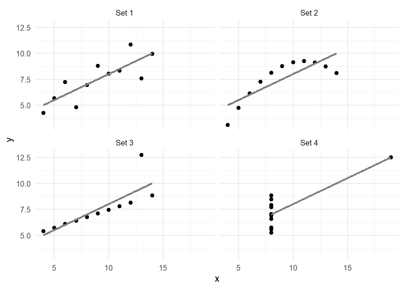
This figure shows why it helps to plot before computing. Anscombe built these four datasets in 1973. One is a clean line with scatter, one is a smooth curve, one is a perfect line spoiled by a single outlier, and one is a vertical stack with a single leverage point. A table of summary statistics cannot tell them apart. A graph can.
Part 2: Statistical analysis for research (Chapters 5–10)
5. From Research Question to Data. This chapter comes before any test. It moves from a topic to a question to a hypothesis, then to measurement, reliability and validity, study designs, samples, and Planning the analysis before the data. A thesis built in the other order tends to find whatever is easiest to find.
One figure from the chapter is a simulation of the null world: what differences between two random groups of 150 students look like when the workshop does nothing.
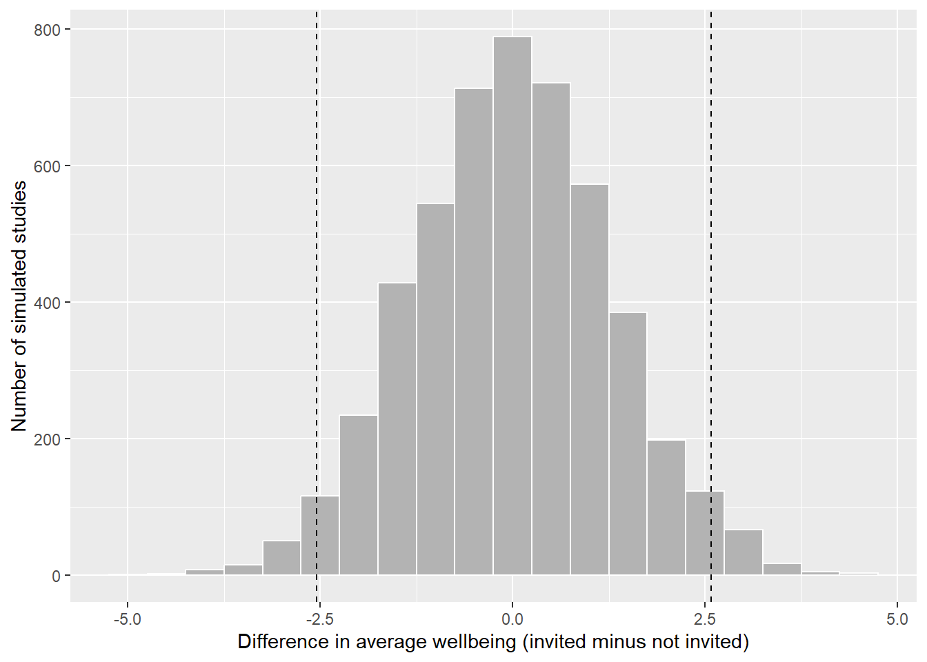
Even when nothing is happening, two groups almost never have identical averages. Chance alone produces differences, usually small ones. That is the intuition a reader needs before the phrase “statistically significant” means anything. The same chapter also separates the roles a third variable can play: a confounder, a moderator, or a mediator.
6. Descriptive Statistics and Exploratory Data Analysis. The title pairs two ideas that beginners often treat as one. Sections on spread, shape, unusual values, and Missing data teach that describing a sample is an act of judgment. Describing your sample in a thesis shows how to turn it into the paragraph an examiner will actually read.
7. Hypothesis Testing and Statistical Inference. I lean on simulation here to make the logic of testing visible. The chapter includes a permutation test, where the workshop labels are shuffled 5,000 times and no shuffle comes close to the observed difference. It also explains power, with a result that is easy to miss: with 10 students per group, a real 5-point effect is detected only about 17% of the time.
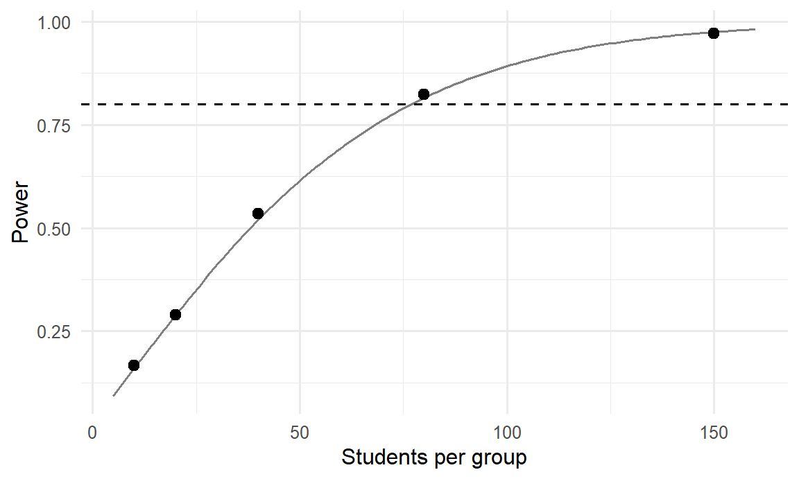
This curve changes how a researcher thinks about “no significant difference”. A small study can fail to find an effect that is truly there. That belongs in a limitations section, and the chapter gives readers the vocabulary to write it.
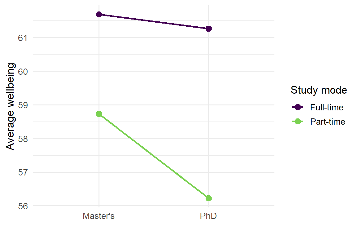
8. ANOVA and Regression. Two-way ANOVA, linear regression, and logistic regression. One figure from this chapter is a plot of an interaction: full-time and part-time students at Master’s and PhD level do not lose wellbeing at the same rate.
9. Multivariate Statistical Methods. The chapter opens with Constructs and latent variables. Stress is not a column you can measure directly, so you measure items and combine them. Principal component analysis, factor analysis, and cluster analysis follow as ways to handle many variables at once.
10. Mixed-Effects Models. Data with a structure names the problem this chapter deals with. Students sit within supervisors, and the same students are measured repeatedly. Treating those observations as independent overstates what you know. Sections on a sleep-deprivation study, change in wellbeing over two years, and students within supervisors give three different structures, and Reporting a mixed-effects model addresses the part most thesis writers struggle with: writing it up.
Part 3: Machine learning with R (Chapters 11–16)
11. Introduction to Machine Learning in R. The main ideas are in the section titles: Generalisation and overfitting, Designing a fair test, and Splitting the data. Prediction is introduced as a question about new students, not the ones you already have, which changes how success is measured.
12. Classification Models. Random forests, k-nearest neighbours, and support vector machines are compared on the same dropout question. Sections such as Comparing models fairly, Choosing the threshold, and Imbalanced outcomes suggest that choosing the algorithm is only part of the work. When an outcome like dropout is rare, a model can score high accuracy while missing most of the students who are actually at risk.
13. Predictive Regression. Predicting final GPA brings regularised regression and boosting, and the section order matters: measure prediction error first, compare models, and only then run The final test. The rule behind that order is that a held-out test set is for one last, honest check, not for choosing between models.
14. Advanced Clustering. What counts as a group is a philosophical question disguised as a section title. Gaussian mixture models and density-based clustering answer it differently, and Evaluating a clustering admits that no single score proves a cluster is real.
15. Neural Networks. The chapter starts with A single neuron and builds up. When neural networks are worth using asks whether one is needed at all, and deep learning appears as an extension, not as the default.
16. Time Series Forecasting. The case study uses counselling service data. Time series is where the “independent observations” assumption fails most obviously, so this chapter echoes the lesson of Chapter 10 in a different setting.
Part 4: Reproducible research and applications (Chapters 17–19)
17. Reproducible Research. Quarto documents that contain their own analysis, a results chapter in Quarto, interactive dashboards with Shiny, open science, and optional Git. The first section, Reproducibility and credibility, treats the two as the same thing, and it connects back to the first chapter’s case for research written in code.
18. Using AI with R. The chapter begins with The reliability of coding, explains how AI assistants work, and only then shows AI as a coding assistant and as a way to code open-ended answers. Using AI responsibly comes last, so readers can judge a tool’s output against what they already understand.
19. Putting It All Together. The final chapter walks through the shape of a research project: from raw export to clean data, describing the sample, answering the research questions, producing One figure for the thesis, and writing the results chapter. It also includes Challenges every researcher meets, because the process is rarely tidy.
What the book is really teaching
A theme across the chapters is that good statistics depends on honest reporting. Plan before you look. Plot before you summarise. Report what you removed. Test fairly and once. Say what a small sample cannot tell you. The R code makes this concrete, and the chapter reviews, exercises, glossary, and appendix of common errors give a nervous researcher a way to practise it.
The book, playground, slide decks, and downloadable data package are at polla.dev/data2thesis_r.