Time Series Forecasting
Time Series Forecasting
When the order of observations carries information
Chapter 16
Polla Fattah
By the end of today you can
- explain dependence over time, and why forecasts are ranges;
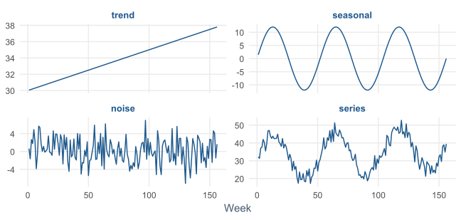
- name the parts of a series: trend, seasonality, noise;
- store a series as a tsibble, and plot it;
- read time plots, seasonal plots, and autocorrelation;
- decompose a series with STL;
- forecast with benchmarks, ETS, and ARIMA in fable;
- evaluate forecasts on a test period, and report prediction intervals.
A different way of thinking
| Survey data | Time series |
|---|---|
| observations independent | this week relates to last week |
| order does not matter | order carries information |
| one value per case | trend, season, and noise together |
A forecast of the future is honestly a range, never a single number.
The counselling service’s question
Five years of weekly visit counts: overwhelmed before exams, quiet in summer, staffing planned by guesswork.
How many visits should the service expect next year, week by week?
An internal analysis, done for the service rather than for publication.
A tsibble knows which column is time
clinic <- tsibble(
  day    = 1:14,
  visits = c(12, 10, 9, 11, 7, 3, 2,   14, 11, 10, 12, 8, 4, 2),
  index  = day
)
Two weeks of daily visits to a small clinic, from a Monday.
The index keeps observations in order and each time unique. Busy early in the week, quiet at the weekend.
Three parts of a pattern
parts <- tibble(
  week     = 1:156,
  trend    = 30 + 0.05 * week,
  seasonal = 12 * sin(2 * pi * week / 52),
  noise    = rnorm(156, sd = 3)
) |>
  mutate(series = trend + seasonal + noise)
An artificial weekly series for three years, built from its parts.
Only the sum is observed
Forecasting extends trend and season. Noise cannot be forecast: the main reason every forecast has a range.
The counselling data as a tsibble
Five academic years, September 2020 to August 2025: 260 weeks.
yearweek() turns each Monday’s date into a week; the header reads [1W].
Plot the series first
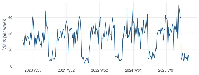
A seasonal pattern each academic year, a gentle upward trend, noise, and one unusual week in autumn 2023.
A seasonal plot
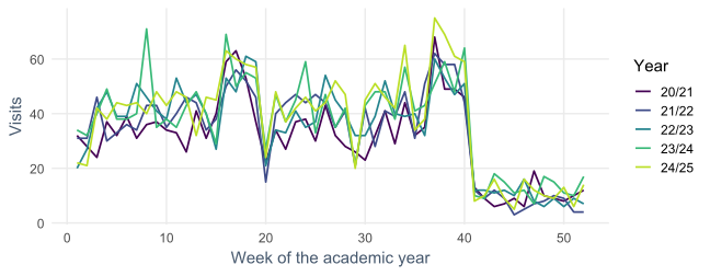
Every year has the same shape; later years lie slightly higher. The period is 52 weeks.
Busy weeks follow busy weeks
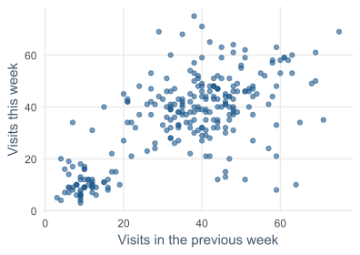
Knowing last week’s visits says a good deal about this week’s.
Autocorrelation
The correlation between the series and itself \(k\) steps earlier.
| Lag | 1 | 26 | 52 |
|---|---|---|---|
| autocorrelation | 0.69 | -0.24 | 0.68 |
A week resembles the same week a year earlier. Half a year apart, a busy term week often meets a quiet summer week.
The autocorrelation function
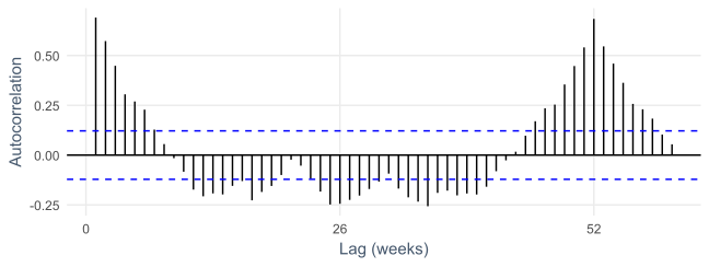
A peak at the seasonal lag is the signature of seasonality. No autocorrelation would mean nothing to forecast beyond the average.
Decomposition with STL
| Component | Is |
|---|---|
| trend | the slow movement |
| seasonal | the repeating academic-year pattern |
| remainder | what is left: the noise |
robust = TRUE stops unusual weeks from distorting trend and season.
The recovered parts
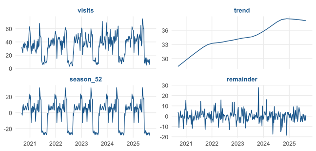
The trend rises from about 28 to 38 visits a week, levelling off in the last year.
The unusual week
visits_stl |> as_tibble() |>
  slice_max(abs(remainder), n = 3) |>
  select(week, visits, trend, season_52, remainder)
The week of 23 October 2023: 71 visits, about 28 more than trend and season predict.
It was the mental health awareness week. A real week, not an error: kept, and the robust fit stops it distorting forecasts.
Growing seasonal swings
The peaks get higher as the trend rises, while the summer lows stay low.
When the season grows with the level, model the logarithm of the series.
In fable, write log(visits) in the model; forecasts are transformed back automatically.
Benchmarks first
| Method | Forecasts |
|---|---|
| mean | the average of all past observations |
| naive | the last observed value |
| seasonal naive | the value from the same season last cycle |
Every forecasting method must beat these, as every model in Chapters 11–13 had to beat a baseline.
Benchmarks on the clinic
clinic |>
  model(mean   = MEAN(visits),
        naive  = NAIVE(visits),
        snaive = SNAIVE(visits ~ lag(7))) |>
forecast(h = 7)| Method | Forecast for next week |
|---|---|
| mean | 8.2 every day |
| naive | 2 every day: a quiet Sunday repeated |
| seasonal naive | last week’s pattern repeated |
Two families of models
| Family | Forecasts with |
|---|---|
| ETS, exponential smoothing | weighted averages, recent weeks counting most; tracks level, trend, season |
| ARIMA | how each value depends on earlier values and shocks |
ETS() and ARIMA() choose their details automatically.
Both work best with short seasons: 4 quarters, 7 days, 12 months. A 52-week season is long.
Two strategies for weekly data
flowchart LR
    A["Weekly series"] --> B["STL: remove<br>the season"] --> C["ETS on the<br>adjusted series"] --> D["Add the<br>season back"]
    A --> E["ARIMA with<br>Fourier waves"]
decomposition_model() does the first in one step. fourier(period = 52, K = 6) uses six pairs of smooth waves.
Training and test periods
visits_train <- visits |> filter(week_start <  as.Date("2024-09-01"))
visits_test  <- visits |> filter(week_start >= as.Date("2024-09-01"))
The test period must come after the training period: a forecast can only use the past.
Train on four academic years, test on the fifth.
Five models at once
visits_fit <- visits_train |>
  model(
    mean    = MEAN(visits),
    naive   = NAIVE(visits),
    snaive  = SNAIVE(visits ~ lag(52)),
    stl_ets = decomposition_model(
                STL(log(visits) ~ season(period = 52), robust = TRUE),
                ETS(season_adjust ~ season("N"))),
fourier = ARIMA(log(visits) ~ fourier(period = 52, K = 6) + PDQ(0, 0, 0)))season("N"): no season inside ETS, it comes from STL. PDQ(0, 0, 0): the Fourier terms handle the season.
Accuracy on the test year
| model | RMSE | MAE |
|---|---|---|
| stl_ets | 7.4 | 5.6 |
| snaive | 9.2 | 7.0 |
| fourier | 10.3 | 7.8 |
| mean | 18.7 | 16.3 |
| naive | 27.5 | 23.5 |
STL with ETS is best. The Fourier model struggles with sharp steps, such as the summer drop from one week to the next.
The two best, against reality
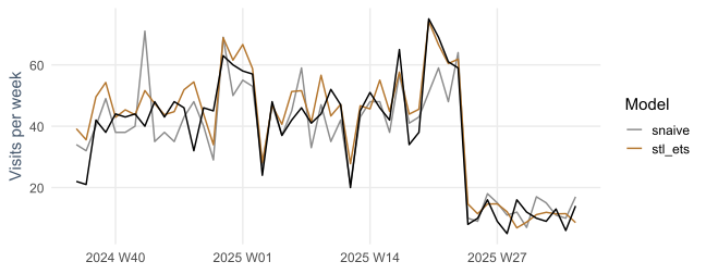
The seasonal naive copies last year’s noise, even the awareness-week spike. STL with ETS is smoother and closer.
Forecasting next year
final_fit <- visits |>
  model(stl_ets = decomposition_model(
    STL(log(visits) ~ season(period = 52), robust = TRUE),
    ETS(season_adjust ~ season("N"))))
next_year <- final_fit |> forecast(h = 52)
Refitted on all five years, so the forecasts use the most recent information.
Prediction intervals
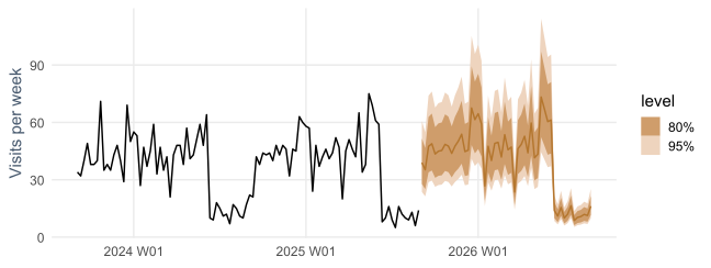
80% and 95% ranges. First week: about 39 visits, anywhere from 24 to 61 unsurprising.
A total for the year needs simulation
set.seed(2026)
futures <- final_fit |> generate(h = 52, times = 1000)
yearly_totals <- futures |> as_tibble() |>
  summarise(total = sum(.sim), .by = .rep)
quantile(yearly_totals$total, c(0.025, 0.5, 0.975))
Weeks do not vary independently, so weekly intervals cannot simply be added.
generate() produces 1,000 possible futures; their totals give the range.
The report to the service
- about 2,111 visits expected in 2025/26 (95% interval 1,952 to 2,286), against 1,954 in 2024/25;
- the busiest weeks will again be just before and during the exam periods;
- an awareness campaign can raise demand sharply for a week: plan extra capacity.
Forecasts assume the future resembles the past
A new booking system, a changed exam calendar, or a crisis like COVID-19 can make any forecast wrong.
- report forecasts with their intervals;
- say what they assume;
- update them as new data arrives.
Prophet, once popular, is no longer actively developed; fable is well supported.
In your field: environmental science
co2_ts |>
  filter(index <= yearmonth("1990 Dec")) |>
  model(snaive = SNAIVE(value), ets = ETS(value), arima = ARIMA(value)) |>
forecast(h = "7 years") |> accuracy(co2_ts)| Model | MAE (ppm) |
|---|---|
| seasonal naive | 5.3 |
| ETS | 1.0 |
| ARIMA | 1.2 |
Mauna Loa CO₂: a strong trend and a 12-month cycle that ETS and ARIMA model directly.
Practical lab: the Chapter 16 playground
Work through the playground exercises in your browser, with hints and solutions.
The browser version builds Fourier terms with lm(); the download uses fable.
Practical exercises 1–4: parts and models
- Which benchmark suits a trend without seasonality? Test it on the clinic.
- Plot the seasonally adjusted series: what does it reveal?
- Fourier terms with
K = 2andK = 12. - Train on three years, test on the fourth.
Practical exercises 5–7: forecasts and communication
- Expected visits in the four weeks before the first exams, with an interval.
- Explain a 95% prediction interval to the service.
- Double the noise in the artificial series: what happens to forecast intervals?
Try this yourself
Find a series in your own field.
- plot it, and name its trend, season, and noise;
- choose the seasonal period;
- pick a benchmark it must beat;
- decide what event could make a forecast wrong.
Troubleshooting guide (Part 1)
| Symptom | Likely cause |
|---|---|
| “duplicated index” error | the same time appears twice |
| ETS or ARIMA struggles with weekly data | the 52-week season is long; decompose first |
| forecasts copy last year’s spikes | seasonal naive repeats the noise |
| one week dominates the trend | use robust = TRUE |
Troubleshooting guide (Part 2)
| Symptom | Likely cause |
|---|---|
| test error suspiciously low | test period not after training period |
| seasonal swings grow with the level | model log() of the series |
| a yearly total without an interval | weekly intervals cannot be added; simulate |
| forecasts wrong after a change | the past no longer resembles the future |
Completion checklist
Misconceptions to leave behind (Part 1)
| Misconception | Better mental model |
|---|---|
| a forecast predicts the exact value | a forecast is a range |
| more history always helps | only if old patterns still hold |
Misconceptions to leave behind (Part 2)
| Misconception | Better mental model |
|---|---|
| any random subset can be the test set | the test period comes after training |
| an unusual week should be removed | keep it; use robust methods |
The chapter in one sentence
Separate trend, season, and noise, beat the simple benchmarks on a later test period, and always report a forecast as a range with its assumptions.
Next: Chapter 17
The next chapter makes research reproducible:
- reproducibility and credibility;
- documents that contain their own analysis;
- a results chapter in Quarto;
- fixed package versions with renv;
- interactive dashboards with Shiny, and open science.
Questions
What regular measurement in your field has a seasonal pattern?
What event could break its forecast?