Classification Models
Classification Models
From predicted probabilities to decisions about people
Chapter 12
Polla Fattah
By the end of today you can
- explain how trees, random forests, k-nearest neighbours, and SVMs classify;
- fit each with tidymodels, and compare them fairly;
- read a confusion matrix;
- calculate sensitivity, specificity, precision, and F1;
- choose a threshold from the costs of the two errors;
- handle an imbalanced outcome, and say what resampling changes.
Two questions about a classifier
- Would more flexible methods rank the cases better than logistic regression?
- What happens when predictions become decisions?
Every decision rule flags some cases wrongly and misses others. The balance depends on what each error costs, and to whom.
Same data, same split, same folds
dropout_split <- initial_split(dropout_data, prop = 0.75,
                               strata = considering_dropout)
dropout_recipe <- recipe(considering_dropout ~ ., data = dropout_train) |>
  step_impute_median(all_numeric_predictors()) |>
  step_dummy(all_nominal_predictors()) |>
  step_normalize(all_numeric_predictors())
dropout_folds <- vfold_cv(dropout_train, v = 10, strata = considering_dropout)
Exactly as in Chapter 11, so every model is trained and tested on the same students.
A decision tree asks questions
tiny_tree <- rpart(dropout ~ stress + support, data = tiny,
                   method = "class",
                   control = rpart.control(minsplit = 2, cp = 0))
Twelve imaginary students, four considering dropout.
- “Is support below 2.75?” puts seven, all “No”, on one side.
- “Is stress 3.1 or more?” separates the rest perfectly.
How a tree chooses its questions
| Term | Meaning |
|---|---|
| node | a question and the students who reached it |
| leaf | a final node, with a predicted class |
| Gini impurity | 0 when a group holds only one class |
The tree tries every predictor and cut-off, and picks the one that makes the groups most pure.
Why trees are attractive
- easy to explain;
- no dummy variables or normalisation needed;
- interactions captured automatically: stress matters only for low-support students.
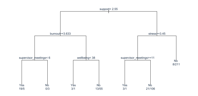
A depth-3 tree for dropout
The first question is about support. Students meeting each condition go left.
A single tree is unstable
A slightly different sample of students can produce a completely different tree.
A deep tree overfits (Chapter 11).
The next method turns this weakness into a strength.
Random forests
- grow hundreds of trees;
- each on a bootstrap sample of the students;
- each split chooses from a random subset of predictors (
mtry); - let the trees vote: P(Yes) is the share voting “Yes”.
Each tree overfits in its own way; many errors cancel. An ensemble of trees.
Fitting a forest
forest_spec <- rand_forest(trees = 500) |>
  set_engine("ranger", importance = "permutation") |>
  set_mode("classification")

forest_wf <- workflow() |>
  add_recipe(tree_recipe) |>
  add_model(forest_spec)
500 trees cannot be drawn: a black box. Permutation importance opens it a little.
What the forest relies on
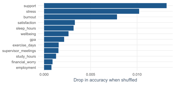
Shuffle one predictor, measure the drop. Importance says what the model uses, not what causes dropout.
k-nearest neighbours
tiny |>
  mutate(distance = sqrt((stress - 3.5)^2 + (support - 3.0)^2)) |>
  arrange(distance) |> head(3)
A new student with stress 3.5 and support 3.0.
The three nearest students vote: two considered dropping out, so P(Yes) = 2/3.
The three nearest neighbours
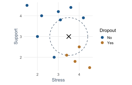
Distances need predictors on one scale: the recipe normalises them.
Tuning k
knn_tuning <- tune_grid(knn_wf, resamples = dropout_folds,
                        grid = tibble(neighbors = c(1, 5, 11, 21, 41, 81)),
metrics = metric_set(roc_auc))| k | 1 | 5 | 11 | 21 | 41 | 81 |
|---|---|---|---|---|---|---|
| AUC | 0.52 | 0.62 | 0.67 | 0.71 | 0.73 | 0.75 |
The smoother k-NN becomes, the better: the pattern in this data is smooth.
Support vector machines
- separate the classes with the widest empty “street”, the margin;
- only the students closest to the boundary, the support vectors, place it;
- overlapping classes: some students may cross, at a cost;
- a kernel lets the boundary bend; the RBF kernel is popular.
Four ways to draw a boundary

Smooth gradient, boxes, patches, rounded regions. All agree: highest risk at high stress and low support.
Comparing six models fairly
dropout_models <- workflow_set(
  preproc = list(tree_data = tree_recipe),
  models  = list(tree = ..., forest = ...)) |>
  bind_rows(workflow_set(
    preproc = list(normalised = dropout_recipe),
    models  = list(logistic = ..., knn = ..., svm_linear = ..., svm_rbf = ...)))

workflow_map(dropout_models, "fit_resamples", resamples = dropout_folds,
             metrics = metric_set(roc_auc), seed = 2026)
Same folds for every model. Trees use the simple recipe, the others the normalised one.
The simple model wins again
| Model | Cross-validated AUC | Std. error |
|---|---|---|
| logistic regression | 0.80 | 0.030 |
| linear SVM | 0.79 | 0.031 |
| random forest | 0.78 | 0.038 |
| RBF SVM | 0.76 | 0.039 |
| k-NN (k = 41) | 0.73 | 0.029 |
| decision tree | 0.73 | 0.025 |
Risk changes smoothly, with no thresholds for a tree to find. Logistic regression is kept, and explained in one sentence.
From ranking to deciding
The AUC measures how well a model ranks students.
The counselling service needs a decision: contact this student or not.
A student is flagged when P(Yes) is above a threshold, 0.5 by default. The confusion matrix counts how the decisions turn out.
The four outcomes
| Truly at risk | Not at risk | Total | |
|---|---|---|---|
| flagged | 8 true positives | 4 false positives | 12 |
| not flagged | 2 false negatives | 86 true negatives | 88 |
| total | 10 | 90 | 100 |
A screening questionnaire given to 100 students, 10 truly at risk.
Measures from the four counts
| Measure | Question | Here |
|---|---|---|
| sensitivity (recall) | how many at risk are found? | 8/10 = 80% |
| specificity | how many not at risk are left alone? | 86/90 = 96% |
| precision | how often is a contact justified? | 8/12 = 67% |
| F1 | precision and recall together | 0.73 |
| accuracy | share classified correctly | 94% |
The study’s model at 0.5
test_results |> conf_mat(truth = considering_dropout, estimate = .pred_class)
class_metrics <- metric_set(accuracy, sensitivity, specificity,
precision, f_meas)| Accuracy | Sensitivity | Specificity | Precision |
|---|---|---|---|
| 83% | 22% | 95% | 42% |
Of 23 at-risk test students, only 5 are flagged. The model ranks well; the threshold is the problem.
0.5 is a default, not a law
| Lower threshold | Higher threshold |
|---|---|
| more students flagged | fewer students flagged |
| higher recall | higher precision |
| more false alarms | more students missed |
Here a flag means a conversation: cheap and harmless. Missing a student who leaves is costly. The threshold belongs well below 0.5.
Choose the threshold without the test set
logistic_cv <- fit_resamples(logistic_wf, resamples = dropout_folds,
                             control = control_resamples(save_pred = TRUE))
cv_predictions <- collect_predictions(logistic_cv)
Cross-validated predictions for every training student, each from a model that did not see them.
The ROC curve
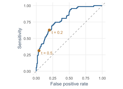
Every threshold at once. The AUC is the area under the curve.
The trade-off in a table
| threshold | flagged | recall | precision | specificity |
|---|---|---|---|---|
| 0.50 | 8% | 31% | 57% | 96% |
| 0.40 | 13% | 40% | 47% | 92% |
| 0.30 | 18% | 49% | 40% | 87% |
| 0.20 | 26% | 63% | 36% | 80% |
| 0.15 | 33% | 72% | 33% | 74% |
| 0.10 | 42% | 75% | 27% | 64% |
map() runs the calculation for each threshold; list_rbind() stacks them.
Costs of the two errors
cost_miss        <- 10   # a student at risk who is not contacted
cost_false_alarm <- 1    # an unnecessary conversation
Costs are judgements about consequences, not statistics. Make them explicit.
The cheapest threshold
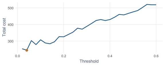
Lowest at about 0.04, flagging 57% of students. Decision theory: \(1 / (1 + 10) \approx 0.09\). Both say: far below 0.5.
The threshold is a decision with an ethical side
- set costs with the people who will use the model;
- state them in the thesis;
- examine the effects on different groups;
- respect practical limits: counsellors cannot see everyone.
The service settles on 0.2: flag about 26%, find about 63% of those at risk, precision about 36%.
Applying 0.2 to the test students
test_results <- test_results |>
  mutate(flag = factor(if_else(.pred_Yes >= 0.2, "Yes", "No"),
                       levels = c("Yes", "No")))
test_results |> class_metrics(truth = considering_dropout, estimate = flag)
The model now finds 13 of 23 at-risk students instead of 5, flagging 35 in all.
Accuracy fell to 79%. It does not matter: accuracy was never the goal.
Report the threshold
Sensitivity, specificity, precision, and F1 all depend on the threshold.
Report which threshold was used, and why.
The AUC does not depend on it, which is why it is used to compare models.
Imbalanced outcomes
| Remedy | How |
|---|---|
| move the threshold | flag at a lower probability |
| upsampling | repeat rare-class students |
| downsampling | drop common-class students |
| SMOTE | create artificial rare-class students |
| class weights | make rare-class mistakes count more |
The themis package adds resampling steps to a recipe.
Upsampling
| Sensitivity at 0.5 | AUC | |
|---|---|---|
| upsampled | 67% | 0.79 |
Resampling applies to training data only. It pushed probabilities up, like lowering the threshold, but did not improve ranking.
After upsampling, a “probability” of 0.6 no longer means a 60% chance.
Does the model work equally well for everyone?
| Test students at risk | Found at 0.2 |
|---|---|
| women: 13 | 7 |
| men: 10 | 6 |
Similar shares, but too few students to detect a difference.
Check sensitivity and precision for every group that matters, on as much data as possible.
In your field: ecology
penguin_wf <- workflow() |>
  add_formula(species ~ bill_length_mm + bill_depth_mm +
                flipper_length_mm + body_mass_g) |>
  add_model(rand_forest(trees = 500) |> set_engine("ranger") |>
              set_mode("classification"))
last_fit(penguin_wf, penguin_split) |> collect_predictions() |>
  conf_mat(truth = species, estimate = .pred_class)
Three penguin species from four measurements: every test penguin classified correctly.
Well-separated classes suit flexible models.
Practical lab: the Chapter 12 playground
Work through the playground exercises in your browser, with hints and solutions.
The browser version builds trees and thresholds with base R and rpart; the download uses tidymodels.
Practical exercises 1–4: models
- A depth-2 tree, explained to a counsellor.
- Tune the forest’s
mtryover 2, 5, and 10. - k-NN with 81, 161, and 301 neighbours: what happens?
- The F1 score of the tiny confusion matrix, by hand.
Practical exercises 5–7: decisions
- Only 10% of students can be contacted: which threshold?
- Downsampling instead of upsampling: sensitivity and AUC?
- A missed student costs 3, not 10: the new cheapest threshold?
Try this yourself
For a classifier in your own field:
- name what a false positive and a false negative mean in practice;
- estimate the cost of each;
- calculate the decision-theory threshold;
- say who should agree to those costs before the model is used.
Troubleshooting guide (Part 1)
| Symptom | Likely cause |
|---|---|
| a tree changes completely between samples | trees are unstable; use a forest |
| k-NN dominated by one variable | predictors not normalised |
| best k at the edge of the grid | extend the grid |
| a flexible model loses | the pattern is smooth |
Troubleshooting guide (Part 2)
| Symptom | Likely cause |
|---|---|
| high accuracy, few cases found | threshold too high for a rare outcome |
| threshold chosen on the test set | the test is spent; use cross-validation |
| sensitivity reported without a threshold | the number cannot be interpreted |
| probabilities too high after upsampling | resampling distorts probabilities |
Completion checklist
Misconceptions to leave behind (Part 1)
| Misconception | Better mental model |
|---|---|
| flexible models always predict better | only when the pattern needs flexibility |
| importance shows cause | importance shows what the model uses |
Misconceptions to leave behind (Part 2)
| Misconception | Better mental model |
|---|---|
| 0.5 is the right threshold | the threshold comes from costs |
| resampling improves a model | it usually shifts probabilities, not ranking |
The chapter in one sentence
Compare models by how well they rank cases, then choose the threshold from what each kind of error costs, and report it.
Next: Chapter 13
The next chapter predicts a number:
- measuring prediction error;
- ordinary regression with many predictors;
- regularised regression: ridge, lasso, elastic net;
- boosting;
- comparing models and the final test.
Questions
In your field, which is worse: a false alarm or a missed case?
Who decides?