Hypothesis Testing and Statistical Inference
Hypothesis Testing and Statistical Inference
From the students we measured to the students we mean
Chapter 7
Polla Fattah
By the end of today you can
- explain a sampling distribution and the standard error;
- calculate and interpret a confidence interval, including a bootstrap interval;
- explain a p-value through a permutation test;
- describe Type I and Type II errors, power, and multiple testing;
- run one-sample, two-sample, and paired t-tests;
- measure the size of an effect with Cohen’s d;
- judge assumptions and choose a non-parametric test when they fail;
- test categorical relationships with chi-square tests;
- report a test in a thesis.
Two research questions from Chapter 5
RQ2: do graduate students sleep less than the recommended 7 hours?
RQ3: did the wellbeing workshop improve wellbeing?
Both are questions about all graduate students.
The student wellbeing data holds 600 of them.
Population, sample, parameter, statistic
| Term | Meaning | Example |
|---|---|---|
| population | everyone the conclusion covers | all graduate students |
| sample | the people actually measured | the 600 students in the data |
| parameter | a number describing the population | true average sleep |
| statistic | the same number from the sample | average sleep of the 600 |
The parameter is never known exactly. The statistic is our estimate of it.
A second sample would disagree
One study shows one estimate.
It cannot show how much that estimate would move if the study were repeated.
A simulation can: treat the 600 students as if they were the population, draw many small samples, and watch the estimates.
Simulating many samples
caffeine <- first_sem$caffeine_mg[!is.na(first_sem$caffeine_mg)]

set.seed(2026)
means_5  <- replicate(1000, mean(sample(caffeine, 5)))
means_30 <- replicate(1000, mean(sample(caffeine, 30)))
sample() draws one random sample; replicate() repeats the whole step.
set.seed() makes the “random” samples the same every time the code runs.
A sampling distribution
The distribution of a statistic over many possible samples is its sampling distribution.
Three lessons in one picture
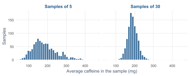
- Both distributions centre on the average of all 600 students, 189 mg: the sample mean is unbiased.
- Averages of 30 are packed far more tightly: larger samples are more precise.
- Caffeine is skewed, yet averages of 30 are nearly bell-shaped.
The third lesson has a name.
The central limit theorem
Whatever the shape of the data, averages of reasonably large samples are approximately normal.
It explains why methods built on the normal distribution work for so many kinds of data.
Rule of thumb: 30 or more is enough unless the data is extremely skewed.
The standard error measures precision
The spread of a sampling distribution is the standard error (SE).
\[ SE = \frac{s}{\sqrt{n}} \]
A real study has one sample, not a thousand. For a mean, the formula recovers the spread from that single sample.
The formula agrees with the simulation
sd(means_30)              # spread of 1,000 simulated averages
sd(caffeine) / sqrt(30)   # the formula, from the data
Here: 25.7 against 26.2 mg.
The square root has a practical cost: halving the SE needs four times as many participants.
A confidence interval adds precision to an estimate
\[ \bar{x} \pm 2 \times SE \]
A 95% confidence interval is a range of plausible values for the parameter.
The “2” is really a value from the t-distribution, and R works it out.
A confidence interval in R
Average sleep is plausibly between 6.40 and 6.57 hours.
The interval is narrow because 600 students is a large sample.
What “95%” describes
flowchart LR
    A["Repeat the study many times"] --> B["Build a 95% interval each time"]
    B --> C["About 95% of intervals contain the true value"]
The confidence belongs to the procedure, not to one interval.
Any single interval either contains the true value or does not.
Mean ± SE is not a confidence interval
mean ± SE      covers roughly 68%
mean ± 2 SE    covers roughly 95%
Theses often report “mean ± SE” as if it were a 95% interval.
Report the confidence interval itself, and say what it is.
Some statistics have no simple formula
The SE formula works for means.
For a median, a ratio, or a correlation, there is often no convenient formula.
The bootstrap replaces the formula with resampling.
The bootstrap resamples the sample
flowchart LR
    S["The one sample"] -->|draw with replacement| R1["Resample 1"]
    S --> R2["Resample 2"]
    S --> R3["... 2,000 resamples"]
    R1 --> D["Distribution of the statistic"]
    R2 --> D
    R3 --> D
Treat the sample as the population. Each resample repeats some people and leaves others out.
A bootstrap interval for a median
set.seed(1)
small_sample <- sample(caffeine, 40)

boot_medians <- replicate(2000,
  median(sample(small_sample, replace = TRUE)))

quantile(boot_medians, c(0.025, 0.975))
replace = TRUE is what makes it a bootstrap.
The middle 95% of the bootstrap medians is the 95% interval.
From “plausible values” to “is this claim consistent?”
A confidence interval says which values are plausible.
A hypothesis test asks a sharper question: is the data consistent with one particular claim?
The null and the alternative
| Hypothesis | Statement | For the workshop |
|---|---|---|
| null, \(H_0\) | nothing is going on | the workshop has no effect |
| alternative, \(H_1\) | the researcher’s expectation | the workshop changes wellbeing |
The test is built around \(H_0\) because it is precise enough to calculate with.
Think before you analyse
| Step | For RQ3 |
|---|---|
| question | does the workshop improve wellbeing? a causal question |
| unit | the student, one score each, end of semester 2 |
| outcome | wellbeing, 0 to 100, interval |
| predictor | invited or not invited, at random |
| evidence against \(H_1\) | a gap near zero, or favouring the not invited |
Decide what would count against you before you see the result.
The observed difference
semester2 <- semesters |>
  filter(semester == 2) |>
  left_join(students, join_by(student_id))

observed_gap <-
  mean(semester2$wellbeing[semester2$workshop == "Invited"]) -
  mean(semester2$wellbeing[semester2$workshop == "Not invited"])
Invited students scored 5.2 points higher.
Is that larger than chance differences usually are?
If \(H_0\) is true, the labels carry no information
Under the null, each student would have the same score whichever label they received.
So the labels can be shuffled among the students and the gap recalculated.
Each shuffle is one difference that chance alone could produce.
Shuffling builds the null distribution
set.seed(2026)
shuffled_gaps <- replicate(5000, {
  shuffled <- sample(semester2$workshop)
  mean(semester2$wellbeing[shuffled == "Invited"]) -
    mean(semester2$wellbeing[shuffled == "Not invited"])
})
sample() without a size shuffles the whole column.
The observed gap against 5,000 shuffles
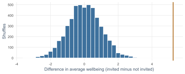
Chance gaps cluster around zero. The observed gap (copper line) is far beyond all of them.
The p-value, by counting
The share of shuffles at least as extreme as the observed gap is the p-value.
Not one of 5,000 shuffles matched it, so we report p < .001, not p = 0.
A test that finds nothing
gpa_gap <- mean(first_sem$gpa[first_sem$gender == "Female"]) -
  mean(first_sem$gpa[first_sem$gender == "Male"])
The same shuffling for GPA by gender: more than half of the shuffles give a gap at least as large.
That gap is exactly what chance produces. There is no reason to reject \(H_0\).
Every test follows the same logic
flowchart TD
    A["Assume H0"] --> B["Work out which results H0 makes likely"]
    B --> C["See where the observed result falls"]
    C --> D["Surprising: reject H0"]
    C --> E["Ordinary: do not reject H0"]
Formal tests replace shuffling with mathematics, and give almost the same answer.
The p-value, stated precisely
The probability of a result at least as extreme as the observed one, if the null hypothesis were true.
Below the significance level, α = 0.05 by convention, the result is called statistically significant.
A large p-value means the data is consistent with \(H_0\). It does not prove \(H_0\).
What a p-value is not
| It is not | It is |
|---|---|
| the probability that \(H_0\) is true | the probability of data like this, assuming \(H_0\) |
| the probability the result is chance | a measure of surprise under \(H_0\) |
| a measure of importance | silent about the size of the effect |
p = 0.03 means: with no workshop effect, a gap this large would appear in 3% of such studies.
Two ways to be wrong
| \(H_0\) really true | \(H_0\) really false | |
|---|---|---|
| reject \(H_0\) | Type I error: false alarm | correct |
| do not reject | correct | Type II error: missed effect |
The significance level controls the first kind. Power controls the second.
Demonstrating the 5% false alarm rate
set.seed(7)
p_values <- replicate(1000, {
  random_group <- sample(rep(c("A", "B"), 300))
  t.test(first_sem$wellbeing ~ random_group)$p.value
})
mean(p_values < 0.05)
The groups are pure chance, yet about 5% of tests come out “significant”.
A single significant result is never the final word.
Power is the chance of finding a real effect
A missed effect depends mainly on:
- the size of the effect;
- the size of the sample;
- the significance level.
Power is the probability that a study detects an effect of a given size when it is real.
Simulating a study
simulate_study <- function(n_per_group, effect = 5, sd = 11) {
  invited     <- rnorm(n_per_group, mean = 60 + effect, sd = sd)
  not_invited <- rnorm(n_per_group, mean = 60, sd = sd)
  t.test(invited, not_invited)$p.value < 0.05
}
Imagine the true workshop effect is 5 points. Run the study 2,000 times per group size and count the successes.
Power grows with the sample
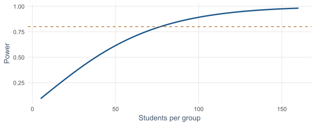
About 80 per group reach 80% power. With 10 per group, the real effect is usually missed.
Read small non-significant studies with caution
10 per group   → power ≈ 0.16
80 per group   → power ≈ 0.80
300 per group  → power ≈ 1.00
“No significant difference” from a small study may describe the study, not the effect.
power.t.test() gives the same curve by calculation.
Many tests, many false alarms
Each test carries its own 5% risk.
With 20 tests of true nulls, the chance of at least one false alarm is about 64%.
Simulating the multiple testing problem
set.seed(8)
any_false_alarm <- replicate(1000, {
  p <- replicate(20, t.test(rnorm(30), rnorm(30))$p.value)
  any(p < 0.05)
})
mean(any_false_alarm)
About two studies in three find “something” in pure noise.
State the main hypotheses in advance, and correct for many comparisons (Chapter 8).
One tail or two
| Test | Looks for | When |
|---|---|---|
| two-tailed | a difference in either direction | the default in R, and in theses |
| one-tailed | one direction only | the other direction is impossible or irrelevant, decided in advance |
One-tailed tests are easier to pass. That is exactly why they need a justification.
Significant is not the same as important
With a large enough sample, a tiny, meaningless difference becomes significant.
Report every result with its size, not only its p-value.
The one-sample t-test
mu is the fixed value to compare against.
The test is two-tailed: \(H_0\) says average sleep is 7 hours. The direction is read from the estimate.
Reading the output
| Part | Value | Meaning |
|---|---|---|
| estimate | 6.48 h | the sample average |
| 95% CI | 6.40 to 6.57 h | excludes 7 |
| t | -12.2 | standard errors from 7 |
| p-value | < 2.2e-16 | far too small to be chance |
Graduate students sleep about half an hour less than recommended.
One value per student
A t-test assumes independent observations.
Using all four semesters would count each student up to four times, as if they were four people.
The result would look more certain than it is. Chapter 10 handles repeated measurements properly.
The two-sample t-test: a small example
A 6-point gap with five students per group gives p ≈ 0.04.
Significant by the usual threshold, but fragile evidence.
Look before you test
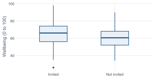
The invited group sits a little higher, but the groups overlap considerably.
Testing the workshop
The formula wellbeing ~ workshop reads “wellbeing by workshop group”.
Gap: 5.2 points, 95% CI 3.4 to 7.1, p < .001, in agreement with the shuffling test.
Randomisation allows a causal conclusion
flowchart TD
    R["Random invitation"] --> A["Groups alike in everything else"]
    A --> B["Only the invitation differs"]
    B --> C["The workshop caused the gap"]
Without random assignment, the same test would show only an association.
Welch is the safe default
The output heading says “Welch Two Sample t-test”.
Welch’s version does not assume the two groups have equal spread.
That makes it the safer choice, and the right default.
How big is five points?
Cohen’s d: the difference between the means, divided by the standard deviation.
It expresses the gap in standard deviations, so it compares across studies and scales.
Interpreting Cohen’s d
| d | Label |
|---|---|
| 0.2 | small |
| 0.5 | medium |
| 0.8 | large |
The workshop: d ≈ 0.45, small to medium.
A real improvement, not a transformation, and worthwhile for a six-week workshop.
The paired t-test compares people with themselves
When the same students are measured twice, the two sets of scores are paired.
Comparing each student with themselves removes the large differences between students.
The test becomes more sensitive.
Paired data needs one row per student
invited_wide <- semesters |>
  filter(semester %in% c(1, 2)) |>
  left_join(students, join_by(student_id)) |>
  filter(workshop == "Invited") |>
  select(student_id, semester, wellbeing) |>
  pivot_wider(names_from = semester, values_from = wellbeing,
              names_prefix = "semester_")

t.test(invited_wide$semester_2, invited_wide$semester_1, paired = TRUE)
A paired test cannot say why
flowchart TD
    A["Invited students improved"] --> B["The workshop worked?"]
    A --> C["Semester 2 was easier for everyone?"]
The paired test has no comparison group.
The two-sample test, invited against not invited, answers the causal question.
The assumptions of the t-test
| Assumption | How to check |
|---|---|
| independence | the study design; one value per person |
| approximate normality | histogram and Q-Q plot; matters little with 30+ per group |
| similar spread | only for the classic test; Welch does not need it |
Independence cannot be tested. It must be secured when the data is collected.
The trap in normality tests
Shapiro-Wilk says sleep is not normal, yet its histogram looked almost perfectly normal.
With 600 students the test detects tiny, harmless departures.
In small samples, where normality matters, it misses real problems. Trust the graphs.
Non-parametric tests compare ranks
When data is skewed and the sample small, or the data is ordinal, compare ranks instead of values.
Extreme values and skew no longer distort the result.
The price: a little less power when the data is close to normal.
Rank-based replacements
| Parametric | Non-parametric | In R |
|---|---|---|
| two-sample t-test | Mann-Whitney U | wilcox.test(y ~ group) |
| paired t-test | Wilcoxon signed-rank | wilcox.test(x2, x1, paired = TRUE) |
Report medians alongside a rank-based test.
Mann-Whitney on skewed caffeine
tapply(first_sem$caffeine_mg, first_sem$gender, median, na.rm = TRUE)
wilcox.test(caffeine_mg ~ gender, data = first_sem)
The medians differ a little, but p > 0.05: no clear evidence of a difference.
When the two kinds of test agree
The Wilcoxon signed-rank test on the invited students agrees with the paired t-test.
When they agree, either can be reported with confidence.
When they disagree, look at the data again, and trust the test whose assumptions fit.
Chi-square tests compare counts
The t-test compares averages of a number.
The chi-square test (\(\chi^2\)) compares counts in categories against the counts expected under \(H_0\).
Goodness of fit: expected proportions
The split is a little uneven, but p is large.
No evidence against 50/50, and a non-significant result is still a result.
Independence: are two categories related?
jobs <- table(students$employment, students$considering_dropout)
prop.table(jobs, margin = 1) |> round(2)
margin = 1 turns counts into proportions within each row.
About a quarter of full-time workers have considered dropping out, against about one in eight of the others.
Testing the relationship
p = .004: students with full-time jobs are more likely to consider dropping out.
An association, not proof of cause: full-time workers may differ in other ways, such as financial pressure.
Check the expected counts
The chi-square test is reliable when every expected count is at least 5.
When some are not, use Fisher’s exact test, fisher.test().
Choosing a test
flowchart TD
  A[What is the outcome?] -->|Numeric| B{How many groups?}
  A -->|Categorical| K[Chi-square test]
  B -->|One, against a value| C[One-sample t-test]
  B -->|Two| D{Same people twice?}
  B -->|Three or more| F[ANOVA, Chapter 8]
  D -->|No| G[Two-sample t-test]
  D -->|Yes| H[Paired t-test]
  G -.->|skewed, small, or ordinal| I[Mann-Whitney U]
  H -.->|skewed, small, or ordinal| J[Wilcoxon signed-rank]
The tests in R
| Question | Test | In R |
|---|---|---|
| a mean equal to a value? | one-sample t | t.test(x, mu = ) |
| two groups differ? | two-sample t | t.test(y ~ group) |
| same people differ? | paired t | t.test(x2, x1, paired = TRUE) |
| counts match proportions? | goodness of fit | chisq.test(table, p = ) |
| two categories related? | independence | chisq.test(table) |
What a report contains
- the statistic and its degrees of freedom;
- the p-value: exact to two or three decimals, or p < .001;
- the size of the effect with a confidence interval;
- a return to the hypothesis stated in advance.
The effect size matters most.
Writing it up
Invited students reported higher wellbeing (M = 65.5) than those not invited (M = 60.2), a difference of 5.2 points, 95% CI [3.4, 7.1], t(598) = 5.47, p < .001, d = 0.45.
Fill numbers in with code, so they cannot drift from the analysis.
In your field: health research
drug1 <- sleep$extra[sleep$group == 1]
drug2 <- sleep$extra[sleep$group == 2]
t.test(drug2, drug1, paired = TRUE)
The t-test was invented for small medical experiments. The sleep data: 10 patients, two drugs, the same patients on both.
A clear effect of 1.6 hours, but a wide interval from 10 patients.
Practical lab: the Chapter 7 playground
Work through the playground exercises in your browser, with hints and solutions.
The lab rebuilds today’s ideas by hand before using the formal tests.
Practical exercises 1–3: estimates and intervals
- Draw sampling distributions of
study_hoursfor samples of 10 and 50. - Build and interpret a 95% interval for first-semester GPA.
- Test whether average wellbeing differs from 60.
Say in one sentence what each result means.
Practical exercises 4–6: tests and power
- Compare full-time and part-time GPA by shuffling, then by t-test, with Cohen’s d.
- Find the power of 40 per group for a 3-point effect.
- Test whether living away from family is related to considering dropout.
Try this yourself
Choose one comparison in the student wellbeing data that interests you.
- state \(H_0\) and \(H_1\) before looking;
- plot the groups;
- run a permutation test and the matching formal test;
- report the effect size with its interval.
Then explain whether the design allows a causal claim.
Troubleshooting guide (Part 1)
| Symptom | Likely cause |
|---|---|
| results change on every run | no set.seed() before random steps |
| p-value looks too small | the same students counted several times |
| “mean ± SE” in the table | SE mistaken for a confidence interval |
| a significant result in a large study seems trivial | significance mistaken for importance |
Troubleshooting guide (Part 2)
| Symptom | Likely cause |
|---|---|
| Shapiro-Wilk rejects a normal-looking variable | a large sample detects harmless departures |
| a chi-square warning about approximation | expected counts below 5; use fisher.test() |
| a paired test used for two different groups | the design is independent, not paired |
| many tests, one “finding” | multiple testing without correction |
Completion checklist
Misconceptions to leave behind (Part 1)
| Misconception | Better mental model |
|---|---|
| the p-value is the chance \(H_0\) is true | the chance of data this extreme if \(H_0\) is true |
| non-significant means no effect | a small study can miss a real effect |
| significant means important | the effect size answers importance |
Misconceptions to leave behind (Part 2)
| Misconception | Better mental model |
|---|---|
| p = 0.049 and p = 0.051 differ | almost identical evidence |
| normality tests decide if a t-test is allowed | graphs and sample size are the better guide |
| many tests at α = 0.05 are harmless | the risks accumulate |
The chapter in one sentence
A test asks how surprising the data would be if nothing were going on; report how big the effect is, not only whether it is significant.
Next: Chapter 8
The next chapter extends comparisons to:
- three or more groups with ANOVA;
- corrections for multiple comparisons;
- linear regression and adjustment;
- logistic regression for yes-or-no outcomes.
Questions
For your own thesis question, what is \(H_0\)?
What result would count as evidence against your expectation?