flowchart TD
  A["Topic: graduate student wellbeing"] --> B["Problem: many report stress; some leave"]
  B --> C["Focus: can the university do something?"]
  C --> D["Question: does a six-week workshop improve<br>wellbeing by the end of the next semester?"]
From Research Question to Data
From Research Question to Data
Deciding what you are asking before any statistics
Chapter 5
Polla Fattah
By the end of today you can
- explain what data analysis is for: describing, explaining, predicting;
- turn a topic into a focused research question;
- write a falsifiable hypothesis and its null hypothesis;
- turn a construct into a measured variable and judge its level;
- name the roles variables play;
- distinguish reliability from validity;
- say what each study design can and cannot show;
- explain why a biased sample cannot be fixed by making it larger;
- plan an analysis and a sample size before collecting data.
Most thesis problems start before the analysis
- a question too vague to answer;
- a hypothesis no result could contradict;
- a questionnaire that measures something other than the title promises;
- a sample that cannot support the conclusion.
No statistical test can fix these afterwards.
Data analysis tests claims against evidence
| Aim | Example question | Judged by |
|---|---|---|
| describe | how long do graduate students sleep? | accuracy, and who it applies to |
| explain | does the workshop improve wellbeing? | whether rival explanations are ruled out |
| predict | who will consider dropping out? | accuracy on new cases |
Describing: Chapters 4, 6, 7. Explaining: 7 to 10. Predicting: 11 to 16.
The same model, different aims
A regression can explain GPA: which predictors matter, and how much?
It can also predict GPA: how close are the predictions for new students?
The model may be identical. The question, and how the answer is judged, are not.
From a topic to a research question
A research question is a topic narrowed until data can answer it.
A good research question is
- specific: who, what, and when;
- answerable with data you can collect;
- not already answered;
- feasible with your time, money, skills, and access;
- worth answering: someone would act differently.
Weak questions, improved
| Weak | Problem | Better |
|---|---|---|
| Are students stressed? | compared with what? | Do part-time students report higher stress than full-time? |
| What affects success? | “success” undefined | Is sleep associated with GPA, allowing for study hours? |
| Is the workshop good? | “good” is not measurable | Does it raise wellbeing by the end of semester 2? |
| Why do students drop out? | needs years of follow-up | Which baseline traits go with considering dropout? |
Three kinds of question
| Kind | Asks | Needs | Can claim |
|---|---|---|---|
| descriptive | what is? | a representative sample | a summary |
| relational | what goes with what? | both variables measured | association |
| causal | what leads to what? | a design ruling out alternatives | cause |
Asking a relational question and answering in causal words (“sleep improves grades”) is a common error.
A hypothesis answers in advance
Hypothesis: Students invited to the workshop will have higher wellbeing at the end of semester 2 than students not invited.
A research question asks. A hypothesis is the best prediction, from theory and earlier studies.
It is useful because the data can disagree with it.
Falsifiability
| Hypothesis | Could a result contradict it? |
|---|---|
| “The workshop affects students in some way.” | no: unfalsifiable |
| “It helps students who are ready for it.” | no, unless “ready” is defined first |
| “Invited students will have higher wellbeing in semester 2.” | yes: equal or lower wellbeing |
Popper: a scientific claim forbids certain results.
Write down what would count against you
Before seeing any data, name the result that would contradict the hypothesis.
If you cannot, it is not yet precise enough.
If you can, you are protected from explaining away a disappointing result afterwards.
Four properties of a good hypothesis
- about a stated population and stated variables;
- testable with the data available;
- falsifiable: it names the contradicting result;
- stated before the data is analysed.
A hypothesis written after seeing the data describes the data. It does not test it.
Directional and non-directional
| Kind | Predicts | Example |
|---|---|---|
| directional | the direction of an effect | invited students will have higher wellbeing |
| non-directional | only that a difference exists | wellbeing will differ between faculties |
The direction of the hypothesis and a one- or two-tailed test are separate decisions (Chapter 7).
The null hypothesis
| Statement for the workshop | |
|---|---|
| \(H_1\), alternative | invited and not invited differ in average wellbeing |
| \(H_0\), null | they have the same average wellbeing |
\(H_0\) is precise enough to calculate with: any difference is due to chance alone.
Simulating the null world
set.seed(2026)
chance_differences <- replicate(5000, {
  wellbeing <- rnorm(300, mean = 60, sd = 11)
  group     <- sample(rep(c("Invited", "Not invited"), 150))
  mean(wellbeing[group == "Invited"]) -
    mean(wellbeing[group == "Not invited"])
})
300 imaginary students, a workshop that does nothing, two random groups, repeated 5,000 times.
rnorm() draws normal random numbers; sample() shuffles the labels.
Chance alone produces differences
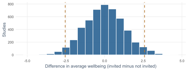
95% of chance differences lie between -2.5 and 2.6. A 5-point gap would be hard to explain by chance; 1 point would not.
What a test can and cannot conclude
- rejecting \(H_0\) is not proving \(H_1\): “nothing is going on” is just a poor explanation;
- not rejecting \(H_0\) is not proving it: a small study can miss a real effect.
A blurred photograph can fail to show a real face.
Confirmatory and exploratory
| Kind | Does | Results |
|---|---|---|
| confirmatory | tests a hypothesis stated in advance | confirm or contradict |
| exploratory | looks for patterns with no prior prediction | suggest future hypotheses |
Both are legitimate, as long as they are labelled honestly.
The study’s questions as hypotheses
| Question | \(H_1\) | Against \(H_1\) |
|---|---|---|
| RQ2 sleep below 7 h? | average sleep < 7 h | interval includes 7 |
| RQ3 workshop helps? | invited higher in semester 2 | gap near zero or negative |
| RQ5 what explains GPA? | more sleep, higher GPA | coefficient near zero |
| RQ8 how does wellbeing change? | it declines over two years | slope near zero or positive |
| RQ9 who considers dropout? | stress raises the odds | odds ratio ≤ 1 |
Descriptive, exploratory, and predictive questions have no null hypothesis.
Think before you analyse
- What is the question: descriptive, relational, or causal?
- What is the unit of analysis: students, semesters, supervisors?
- Which variables, at what level, in which role?
- What result would support the hypothesis, and what would count against it?
Answer in writing before running any code.
The unit of analysis decides what a question means
nrow(students)      # 600: one row per student
nrow(semesters)     # 2326: one row per student per semester
nrow(supervisors)   # one row per supervisor
“Do students who sleep more have higher GPAs?” is about students: each counts once.
2,326 semester rows as independent cases would overstate the evidence (Chapter 10).
Constructs need operationalisation
Stress, wellbeing, motivation: constructs that cannot be observed directly.
Operationalisation decides how to measure one. Every operationalisation is a choice, and another choice could give another answer.
How the study measures its constructs
| Construct | Operationalisation | Variable |
|---|---|---|
| sleep | self-reported hours per night | sleep_hours |
| stress | average of six 1-to-5 items | stress_1 to stress_6 |
| wellbeing | a validated 0-to-100 index | wellbeing |
| performance | semester GPA from records | gpa |
| dropout thoughts | “Have you seriously considered leaving?” | considering_dropout |
Building the stress score
stress <- questionnaire |>
  mutate(stress_4 = 6 - stress_4,
         stress   = rowMeans(pick(stress_1:stress_6), na.rm = TRUE)) |>
  select(student_id, stress)
No single question captures stress, so six are averaged.
stress_4 is worded the other way and is reversed first. This score is the study’s definition of stress.
Self-report is a measurement choice
People overestimate their sleep, underestimate their caffeine, and give expected answers.
Records and devices avoid some problems, at more cost or intrusion.
Every measure has weaknesses. Say what they are.
Levels of measurement
| Level | Values mean | Meaningful summaries | Example |
|---|---|---|---|
| nominal | categories, no order | counts, mode | faculty |
| ordinal | ordered, unknown distances | also median | employment, one item |
| interval | equal distances, no true zero | also mean, SD | wellbeing |
| ratio | equal distances, true zero | also “twice as much” | sleep_hours, caffeine_mg |
The average faculty is meaningless. “Twice as much wellbeing” is too.
R must be told about order
students <- students |>
  mutate(employment = factor(employment,
           levels  = c("None", "Part-time job", "Full-time job"),
           ordered = TRUE))
Alphabetical order puts “Full-time job” before “None”.
An ordered factor fixes tables and graphs, and makes employment > "None" work.
Ordinal numbers are not interval numbers
table(students$financial_worry, useNA = "ifany")
#>   1   2   3   4   5 <NA>
#>  84 139 172 111  56   38
median(students$financial_worry, na.rm = TRUE)
#> [1] 3
“Not at all” to “a little” need not equal “very” to “extremely”. Report the distribution or the median.
Scale scores, averages of several items, are conventionally treated as interval.
The roles variables play
| Role | Meaning | Example |
|---|---|---|
| outcome | what is explained or predicted | wellbeing, GPA |
| predictor | what explains or predicts it | workshop, sleep |
| confounder | related to both; can fake an association | sleep, for caffeine and GPA |
| moderator | changes the strength of a relationship | programme |
| mediator | how the predictor has its effect | lower stress |
Roles come from the question, not the variable.
Three roles of a third variable
flowchart LR
  subgraph Confounder
    S1[Sleep] --> C1[Caffeine]
    S1 --> G1[GPA]
    C1 -. "apparent link" .- G1
  end
  subgraph Mediator
    W[Workshop] --> ST[Lower stress] --> WB[Wellbeing]
  end
A moderator, such as programme, changes the effect of support on GPA.
A confounder in the data
| caffeine | sleep | GPA | |
|---|---|---|---|
| caffeine | 1 | −0.64 | −0.18 |
| sleep | −0.64 | 1 | 0.25 |
More caffeine goes with lower GPA, but also with much less sleep. Chapter 8 compares students with the same sleep.
Reliability and validity
| Property | Question | Stress example |
|---|---|---|
| reliability | is it consistent? | a similar score next week; items agree |
| validity | does it measure the right thing? | stress, not tiredness on the day |
Shots at a target
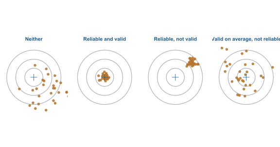
Reliability is necessary for validity, but not enough: a scale always two kilograms too heavy is reliable and wrong.
Kinds of reliability
| Kind | Asks | Measured with |
|---|---|---|
| internal consistency | do a scale’s items agree? | Cronbach’s alpha (Chapter 9) |
| test-retest | same person, same score later? | correlation over time |
| inter-rater | do two coders agree? | Cohen’s kappa (Chapter 18) |
Kinds of validity for a measure
- content validity: do the items cover the whole construct?
- construct validity: does the score behave as the construct should?
- convergent: correlates with related constructs;
- discriminant: correlates less with unrelated ones.
Checking construct validity
| stress | burnout | support | satisfaction | |
|---|---|---|---|---|
| stress | 1 | 0.65 | −0.33 | −0.41 |
Related to burnout, but far from identical; negative with support and satisfaction.
Not proof, but the kind of evidence a thesis reports. Chapter 9 tests the whole questionnaire.
Validity of a whole study
| Kind | Concerns | Depends on |
|---|---|---|
| internal validity | ruling out other explanations | the design |
| external validity | who else the results apply to | the sample |
Study designs
| Design | Can it show cause? | In the study |
|---|---|---|
| randomised experiment | yes, for the treatment | the workshop invitation |
| quasi-experiment | only with care | students who chose many sessions |
| cross-sectional | no, association only | the baseline questionnaire |
| longitudinal | order, still association | the four semesters |
The design, not the statistics, decides whether a study can show cause.
Self-selection confounds
If the workshop were open to volunteers, those who came might already have more energy and less stress.
Any later difference would mix the workshop’s effect with who they already were.
Simulating volunteers against random invitation
chance_to_volunteer <- plogis(-2 * (stress_scores - mean(stress_scores)))
volunteered <- runif(600) < chance_to_volunteer
invited <- sample(rep(c(TRUE, FALSE), 300))| Design | Stress gap before any workshop |
|---|---|
| volunteers | −0.80 |
| random invitation | 0.06 |
plogis() turns a number into a probability; runif() draws a uniform random number.
Randomisation balances what you did not measure
| Group | n | age | % female | % PhD | money worry | stress |
|---|---|---|---|---|---|---|
| invited | 300 | 29.6 | 50.3 | 28.7 | 2.8 | 3.2 |
| not invited | 300 | 29.8 | 53.7 | 29.3 | 2.9 | 3.2 |
Motivation, family support, health: all balanced by chance.
A balance table like this belongs in any thesis with an experiment.
Randomisation is about the treatment only
The random invitation supports causal claims about the invitation, nothing else.
- sleep, stress, caffeine, and GPA are observational;
- what was randomised is the invitation, not attendance;
- comparing students by sessions attended is a quasi-experiment again.
Cross-sectional and longitudinal
| Design | Strength | Weakness |
|---|---|---|
| cross-sectional | quick and cheap | cannot show which came first |
| longitudinal | shows change and order | attrition: people leave |
Those who leave are rarely a random selection.
Ways to draw a sample
| Method | How | Note |
|---|---|---|
| simple random | everyone equally likely | needs a sampling frame |
| stratified | random within groups | every group represented |
| cluster | whole groups sampled | members alike (Chapter 10) |
| convenience | whoever is easy to reach | weakest for generalising |
Random error and bias
| Error | Cause | Larger sample |
|---|---|---|
| random error | which people happened to be chosen | shrinks it |
| bias | the method favours certain people | does nothing |
Simulating a voluntary survey
population <- first_sem$wellbeing
chance_to_answer <- plogis((population - mean(population)) / 10)

sample(length(population), n)                          # random
sample(length(population), n, prob = chance_to_answer) # voluntary
Students with higher wellbeing are more likely to answer, a common pattern.
The true average first-semester wellbeing is 60.5.
A biased sample cannot be fixed by making it bigger
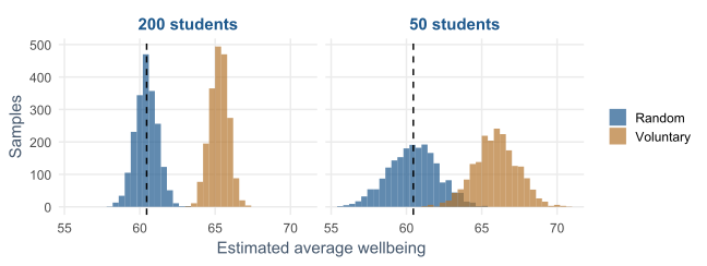
Larger samples are narrower; the voluntary estimate misses just as much.
Attrition in the real data
Of the 37 students who left after year 1, 59% had considered dropping out, against 12% of those who stayed.
Semesters 3 and 4 describe a group less likely to be struggling (Chapters 6 and 10).
Generalising from the sample
The sample: graduate students at one university who agreed to take part.
The results apply most directly there, and elsewhere only by argument.
Claiming less than the data allows is rarely criticised; claiming more is.
An analysis plan
| Hypothesis | Outcome | Analysis | Support if |
|---|---|---|---|
| sleep below 7 h | sleep_hours |
one-sample t-test | interval below 7 |
| workshop raises wellbeing | wellbeing |
two-sample t-test; mixed model | interval excludes 0 |
| stress raises dropout odds | considering_dropout |
logistic regression | odds ratio interval above 1 |
Written before collecting data, it checks that you will collect everything you need.
Power depends on three things
- the sample size;
- the size of the effect, often as Cohen’s d;
- the significance level.
Power is the probability of detecting an effect of a given size if it is real. A common target is 80%.
How many students?
Earlier studies suggest brief programmes improve wellbeing by about 0.4 to 0.5 standard deviations.
About 79 students per group are needed, well below the study’s 300.
Small effects need large samples
sapply(c(small = 0.2, medium = 0.5, large = 0.8),
       \(d) ceiling(power.t.test(delta = d, power = 0.80)$n))
#>  small medium  large
#>    394     64     26
Halving the effect roughly quadruples the sample.
A small study of a small effect cannot say much when it finds nothing.
Preregistration
Exclusions, controls, outliers, choice of test: made after seeing the data, each can drift towards the hoped-for result.
Preregistration writes the hypotheses and plan down, dated, before the analysis.
It does not forbid exploring. It shows which results were predicted and which were found.
Ethics
Research with people needs ethical approval before data collection.
The committee asks the same questions: what the question is, why the data is needed, how participants are recruited, informed, and protected.
A clear question and plan justify collecting only the data you need.
Writing it up
Design. A two-year longitudinal study with an embedded randomised experiment. Participants. 600 graduate students from 5 faculties; 37 (6%) left after the first year. Analysis. With 300 students per group, the workshop comparison had 80% power to detect d = 0.23 at α = .05.
Design, Participants, Measures, and Analysis are the usual headings.
In your field: a laboratory experiment
Sixty guinea pigs, three doses, two delivery methods, ten per combination.
Hypothesis: at the same dose, orange juice produces longer tooth cells than ascorbic acid. With ten per group, only large effects can be detected reliably.
Practical lab: the Chapter 5 playground
Work through the playground exercises in your browser, with hints and solutions.
Every exercise also runs in RStudio, from the downloadable chapter project.
Practical exercises 1–3: questions and measurement
- Improve two vague research questions, and classify each.
- Write a falsifiable hypothesis, its null, and the result against it.
- Give each variable’s level, and make
financial_worryan ordered factor.
Practical exercises 4–6: simulation and planning
- Rerun the null world with groups of 30: how wide are chance differences now?
- Check the invitation’s balance on three more baseline variables.
- Find the sample size for d = 0.3 at 80% and 90% power.
Try this yourself
Take your own thesis topic.
- narrow it to one specific research question;
- classify it as descriptive, relational, or causal;
- write \(H_1\), \(H_0\), and the result that would count against you;
- list each variable with its level and role;
- estimate the sample size you would need.
Troubleshooting guide (Part 1)
| Symptom | Likely cause |
|---|---|
| no result could disprove the hypothesis | it is not falsifiable yet |
| causal words for a correlation | a relational question answered causally |
| categories appear alphabetically | an ordinal variable not declared ordered |
| an average of an ordinal item | the level of measurement ignored |
Troubleshooting guide (Part 2)
| Symptom | Likely cause |
|---|---|
| evidence looks too strong | semester rows treated as independent students |
| groups differed before the treatment | self-selection instead of randomisation |
| a large sample, a wrong answer | a biased sampling method |
| “no significant effect” from 20 people | a study without power |
Completion checklist
Misconceptions to leave behind (Part 1)
| Misconception | Better mental model |
|---|---|
| a hypothesis is a question | it is a prediction precise enough to be wrong |
| rejecting \(H_0\) proves my hypothesis | it rules out only “nothing is going on” |
| non-significant means no effect | the study may have been too small |
Misconceptions to leave behind (Part 2)
| Misconception | Better mental model |
|---|---|
| a big sample is representative | size reduces random error, not bias |
| if it is a number, I can average it | the level of measurement decides |
| a reliable measure is valid | it can be consistent and wrong |
| controlling for variables proves cause | only randomisation balances the unmeasured |
The chapter in one sentence
Decide what you are asking, what result would prove you wrong, and whether your design and sample can answer, before you look at the data.
Next: Chapter 6
The next chapter describes the data:
- the centre, spread, and shape of a distribution;
- unusual values, and why not to delete them;
- missing data and attrition;
- relationships between variables;
- describing the sample in a thesis.
Questions
What would count as evidence against the main hypothesis of your thesis?
Could your design tell that result apart from chance?