By the end of today you can

• explain how a neuron combines its inputs;
• explain why a single sigmoid neuron is a logistic regression;
• describe layers, weights, activation functions, and training;
• fit and tune a network with scikit-learn (MLPClassifier), using weight decay;
• compare a network fairly with simpler models;
• say when deep learning is, and is not, the right tool.

A claim worth testing

“A neural network would surely predict better than logistic regression.”

Neural networks power image recognition, speech, translation, and large language models.

On a table of research data, the claim should be tested, not accepted.

A single neuron

Two inputs, stress and support, with weights 1.2 and −0.8, and a bias of −4.

Working one neuron by hand

For a student with stress 4 and support 2:

\[ -4 + 1.2 \times 4 - 0.8 \times 2 = -0.8 \]

The sigmoid squeezes any number into 0 to 1:

\[ \text{sigmoid}(z) = \frac{1}{1 + e^{-z}} \]

The neuron in Python

def sigmoid(z):
    return 1 / (1 + np.exp(-z))

def neuron(stress, support):
    return sigmoid(-4 + 1.2 * stress - 0.8 * support)

neuron(stress=4, support=2)   # -> 0.31
neuron(stress=2, support=4)   # -> 0.008

A single neuron is a logistic regression

Everything a single neuron can do, Chapter 8 has already done.

From neurons to networks

flowchart LR
  I1((Stress)) --> H1((H1))
  I1 --> H2((H2))
  I1 --> H3((H3))
  I2((Support)) --> H1
  I2 --> H2
  I2 --> H3
  I3((Sleep)) --> H1
  I3 --> H2
  I3 --> H3
  H1 --> O((P of<br>dropout))
  H2 --> O
  H3 --> O

A multilayer perceptron: inputs, a hidden layer, an output. Every arrow is a weight.

Why layers add power

• each hidden neuron learns its own combination of inputs;
• the output neuron combines those;
• curved activations let the network represent curves and interactions.

With enough hidden neurons, a network can approximate almost any relationship. That flexibility is its strength, and its danger.

Two activation functions

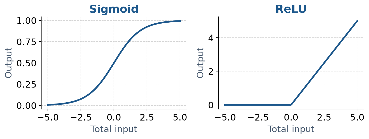
The sigmoid squeezes into 0 to 1. The ReLU zeroes negatives and is standard in deep networks.

How a network learns

• start with small random weights;
• for every weight, find whether a small change would reduce the error: the gradient;
• move all weights a little in the helpful direction: gradient descent;
• one pass through the data is an epoch; training runs for hundreds.

Six students, one neuron

six = pd.DataFrame({
    'stress':  np.array([2.0, 2.5, 3.0, 3.5, 4.0, 4.5]) - 3.25,
    'dropout': np.array([0,   0,   1,   0,   1,   1])
})

Stress is measured from the group’s average.

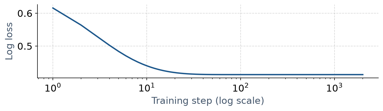
The error to reduce is the log loss: small when high probabilities go to students who did consider dropping out.

Starting from zero

def log_loss(b0, b1):
    p = sigmoid(b0 + b1 * six['stress'])
    return -np.mean(six['dropout'] * np.log(p) + (1 - six['dropout']) * np.log(1 - p))

log_loss(0, 0)   # -> 0.693

With both weights at zero, every student gets a probability of 0.5.

The gradient

p = sigmoid(b0 + b1 * six['stress'])
gradient_b0 = np.mean(p - six['dropout'])
gradient_b1 = np.mean((p - six['dropout']) * six['stress'])

The average prediction error, multiplied by the weight’s input (1 for the bias).

The stress gradient is -0.583: negative, so increasing the weight would reduce the error.

One step of gradient descent

learning_rate = 1.0
b0 = b0 - learning_rate * gradient_b0
b1 = b1 - learning_rate * gradient_b1

Training is nothing more than this step, repeated.

2,000 steps

Two consequences

• training starts from random weights, so two runs differ: random_state matters;
• many weights can keep reducing training error by memorising noise.

Weight decay penalises large weights, exactly like the ridge penalty of Chapter 13. In scikit-learn, this hyperparameter is alpha.

Backpropagation calculates gradients efficiently for thousands of weights.

A network for the dropout question

MLPClassifier(
    hidden_layer_sizes=(10,),
    alpha=3.16,
    max_iter=500,
    random_state=2026
)

Same data, split, ColumnTransformer pipeline, and StratifiedKFold cross-validation as Chapters 11 and 12.

Networks need normalised inputs; StandardScaler provides them.

A network that memorises

big_net = Pipeline([
    ('prep', dropout_recipe),
    ('mlp', MLPClassifier(hidden_layer_sizes=(20,), alpha=0.0, max_iter=1000, random_state=2026, solver='lbfgs'))
])
big_net.fit(X_train, y_train)

Roughly 500 weights for 449 training students: more than enough freedom to memorise every one.

Tuning size and weight decay

param_grid = {
    'mlp__hidden_layer_sizes': [(1,), (3,), (5,), (10,), (20,)],
    'mlp__alpha': [0.01, 0.0316, 0.1, 0.316, 1.0, 3.16, 10.0, 31.6]
}
grid = GridSearchCV(net_pipe, param_grid, cv=dropout_folds, scoring='roc_auc')

Weight decay on a log scale from 0.01 to about 30.

The penalty matters more than the size

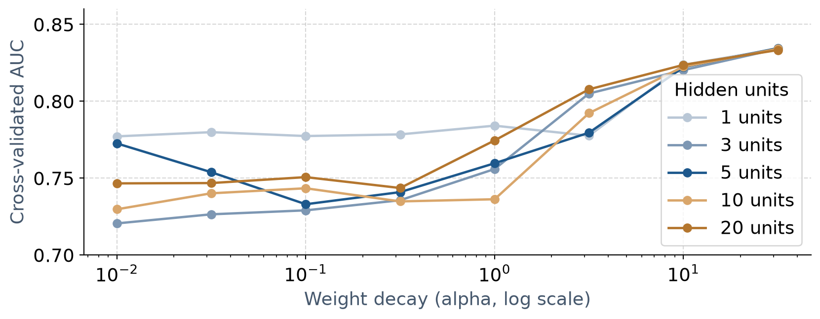
Little decay: networks overfit, the big ones most. Enough decay: every size does about equally well.

A fair comparison

With 150 test students (29 at risk), this difference is well within chance.

A neural network does not predict dropout better.

The costs of the network

• dozens of weights that cannot be interpreted: no odds ratios;
• results depend on random starting weights without strong decay;
• careful tuning needed to avoid overfitting.

Logistic regression is kept. Reporting that a network was tried and did not help is itself a finding.

When neural networks are worth using

A table of a few hundred cases and a few dozen variables, the typical thesis, rarely qualifies.

Deep learning

• many hidden layers, millions or billions of weights;
• each layer builds on the last: edges, then shapes, then objects;
• convolutional networks (CNNs) for images, transformers for text;
• large language models (Chapter 18) are transformers with billions of weights.

Deep learning in Python

For most researchers, the practical route is a pretrained model, as Chapter 18 does with a language model.

In your field: engineering

c_scaler = StandardScaler()
cX_train_s = c_scaler.fit_transform(cX_train)
c_net = MLPRegressor(hidden_layer_sizes=(10,), alpha=0.1, max_iter=2000, random_state=1, solver='lbfgs')

Curves and interactions give the network’s flexibility something to capture.

Practical lab: the Chapter 15 playground

Work through the playground exercises in your browser, with hints and solutions.

Run interactive Python code powered by Pyodide; download the complete offline project.

Practical exercises 1–3: neurons and networks

1. Double the importance of support in the neuron: what does a negative weight mean?
2. One hidden neuron with decay 1.0 against logistic regression.
3. Three seeds with decay 0.01 and with decay 3.16: when does the seed matter?

Practical exercises 4–6: training

4. The 20-neuron network for 10, 100, and 1000 epochs.
5. Explain to the research group why the thesis keeps logistic regression.
6. Gradient descent with learning rates 0.1, 10, and 100: what goes wrong?

Try this yourself

Someone suggests “just use AI” for your prediction problem.

• how many cases and variables do you have?
• is the data a table, or images, sound, or text?
• what simple model would you compare against?
• what would you lose in interpretability?

Troubleshooting guide (Part 1)

Troubleshooting guide (Part 2)

Completion checklist

• a simple model is fitted first as the benchmark;
• inputs are scaled with StandardScaler;
• hidden units and weight decay (alpha) are tuned by cross-validation;
• random_state is set and reported;
• training and test performance are both reported;
• the comparison with the benchmark is fair;
• the loss in interpretability is weighed.

Misconceptions to leave behind (Part 1)

Misconceptions to leave behind (Part 2)

The chapter in one sentence

A neural network is logistic regression units stacked in layers and trained by small steps; it earns its complexity on large, unstructured, or strongly non-linear data, not on every table.

Next: Chapter 16

The next chapter turns to data ordered in time:

• time series data and its components;
• the counselling service’s weekly visits;
• decomposition into trend and seasonality;
• forecasting, and judging forecasts;
• what forecasts assume about the future.

Questions

What would convince you that a neural network is worth its cost?

What would you report if it were not?