ANOVA and Regression
ANOVA and Regression
How much of the variation can other variables explain?
Chapter 8
Polla Fattah
By the end of today you can
- explain how ANOVA splits variation, and what F compares;
- compare three or more groups, and find which differ;
- analyse two factors and their interaction;
- fit and interpret simple and multiple linear regression;
- separate a real effect from a confounder;
- model curves and interactions;
- read diagnostic plots;
- interpret logistic regression as odds ratios and probabilities;
- report ANOVA and regression in a thesis.
Three research questions from Chapter 5
RQ4: does stress differ between faculties and study modes?
RQ5: what explains students' grades?
RQ9: who considers dropping out?
Each asks how an outcome varies with other variables.
ANOVA and regression are the tools for answering them.
The trap in testing every pair
Five faculties give 10 pairs.
Each test has a 5% false alarm risk, and across 10 independent tests the chance of at least one is about 40%.
ANOVA asks one question first: do the faculty averages differ at all?
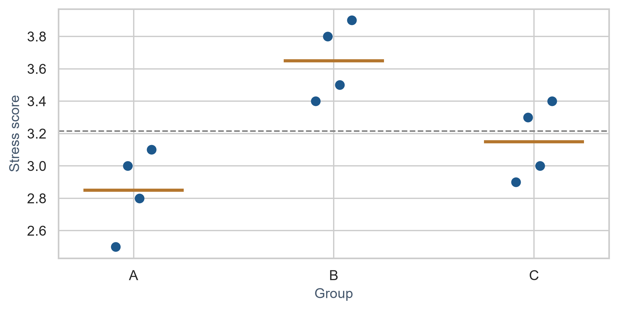
Variation between and within groups
Group averages (copper) vs overall average: between. Points vs their own average: within.
The F statistic
\[ F = \frac{\text{variation between groups}}{\text{variation within groups}} \]
import statsmodels.api as sm
import statsmodels.formula.api as smf

model_group = smf.ols("stress ~ C(group)", data=group_scores).fit()
print(sm.stats.anova_lm(model_group, typ=1))
F near 1: averages differ no more than chance produces. Large F: they differ more.
The ratio matters, not only the gaps
offsets = np.tile([-0.3, -0.1, 0.1, 0.3], 3)
group_avg = np.repeat(group_means.values, 4)

tight = group_scores.assign(stress=group_avg + 0.5 * offsets)
wide = group_scores.assign(stress=group_avg + 4.0 * offsets)| Version | Group averages | F |
|---|---|---|
| tight | identical | 42.8 |
| wide | identical | 0.7 |
Half a point is convincing when students within a group hardly differ, and unremarkable when they differ by two.
Stress by faculty
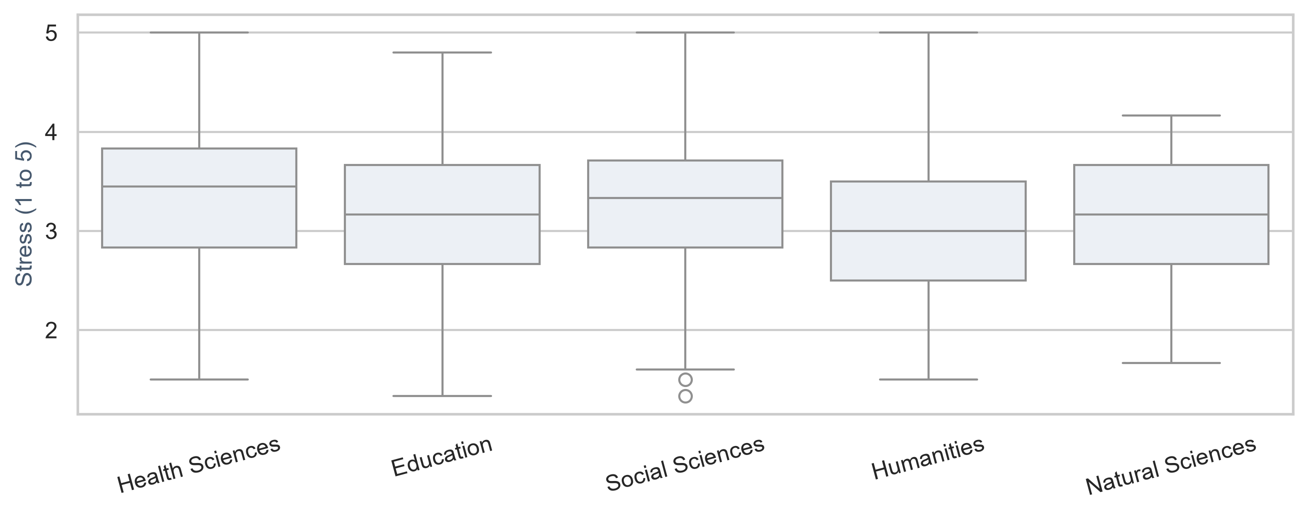
Much overlap. Health Sciences sits a little higher, Humanities a little lower.
One-way ANOVA
stress_anova = smf.ols("stress ~ C(faculty)", data=study).fit()
aov_table = sm.stats.anova_lm(stress_anova, typ=1)
print(aov_table)
\(F(4, 595) = 4.15, p = 0.003\): the faculties differ significantly in stress.
The next question is how much.
Eta squared: the size of the effect
ss_between = aov_table.loc["C(faculty)", "sum_sq"]
ss_total = aov_table["sum_sq"].sum()
eta_sq = ss_between / ss_total
print(f"Eta squared: {eta_sq:.3f}")
\(\eta^2 \approx 0.027\): only about 3% of the differences in stress lie between faculties.
| \(\eta^2\) | 0.01 | 0.06 | 0.14 |
|---|---|---|---|
| guideline | small | medium | large |
Faculty matters, but says very little about one student’s stress.
Post-hoc tests: which groups differ?
from statsmodels.stats.multicomp import pairwise_tukeyhsd

tukey = pairwise_tukeyhsd(endog=study["stress"], groups=study["faculty"], alpha=0.05)
print(tukey)
Tukey’s HSD compares every pair while keeping the overall false alarm rate at 5%.
Only one pair differs: Health Sciences is 0.34 points more stressed than Humanities (\(p = 0.004\)).
Assumptions of ANOVA
| Assumption | How to check | In Python |
|---|---|---|
| independent observations | study design | design stage |
| roughly normal in each group | histograms / Q-Q plots | scipy.stats.probplot |
| similar spread (homoscedasticity) | Levene’s test | scipy.stats.levene(*groups) |
Kruskal-Wallis compares ranks when assumptions fail (\(p = 0.003\), agrees with ANOVA).
Two-way ANOVA
| Term | Meaning |
|---|---|
| main effect of programme | Master’s vs PhD, on average |
| main effect of study mode | full-time vs part-time, on average |
| interaction | does the study-mode effect depend on programme? |
An interaction plot
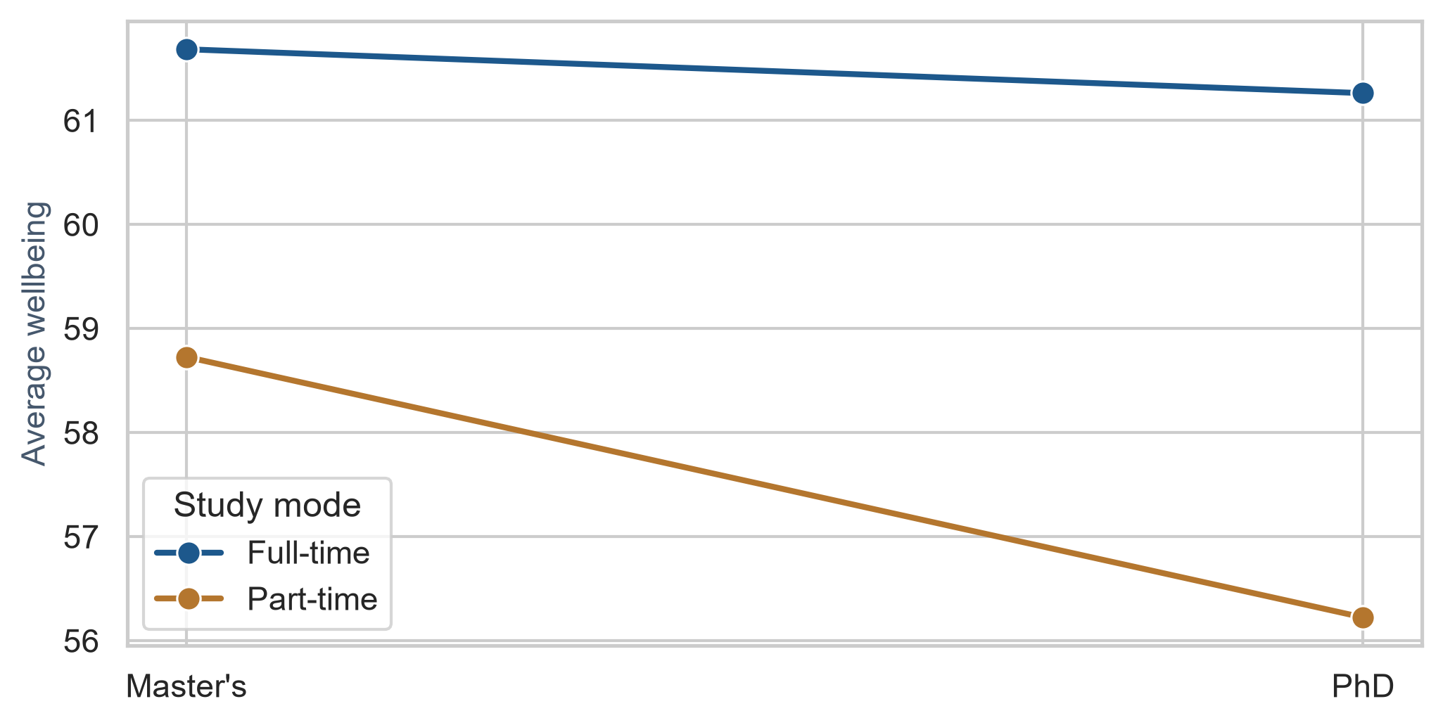
Parallel lines: no interaction. Part-time is lower in both programmes.
Testing main effects and interaction
model_2way = smf.ols("wellbeing ~ C(programme) * C(study_mode)", data=study).fit()
print(sm.stats.anova_lm(model_2way, typ=2))
C(programme) * C(study_mode) requests both main effects and their interaction.
Study mode matters (\(p < .001\)); programme (\(p = 0.29\)) and interaction (\(p = 0.36\)) do not.
A significant interaction is always interpreted before main effects.
Regression models the average outcome
ANOVA compares discrete groups. Regression models how an outcome changes with continuous or categorical predictors.
ANOVA is mathematically a special case of regression.
Average GPA at each level of sleep
sleep_bands = (
    study.dropna(subset=["sleep_hours"])
    .assign(sleep_band=lambda d: (d["sleep_hours"] * 2).round() / 2)
    .groupby("sleep_band")
    .agg(mean_gpa=("gpa", "mean"), students=("student_id", "count"))
    .reset_index()
)
The average GPA of students who sleep 5 hours, 5.5 hours, 6 hours, and so on.
The line summarises conditional averages
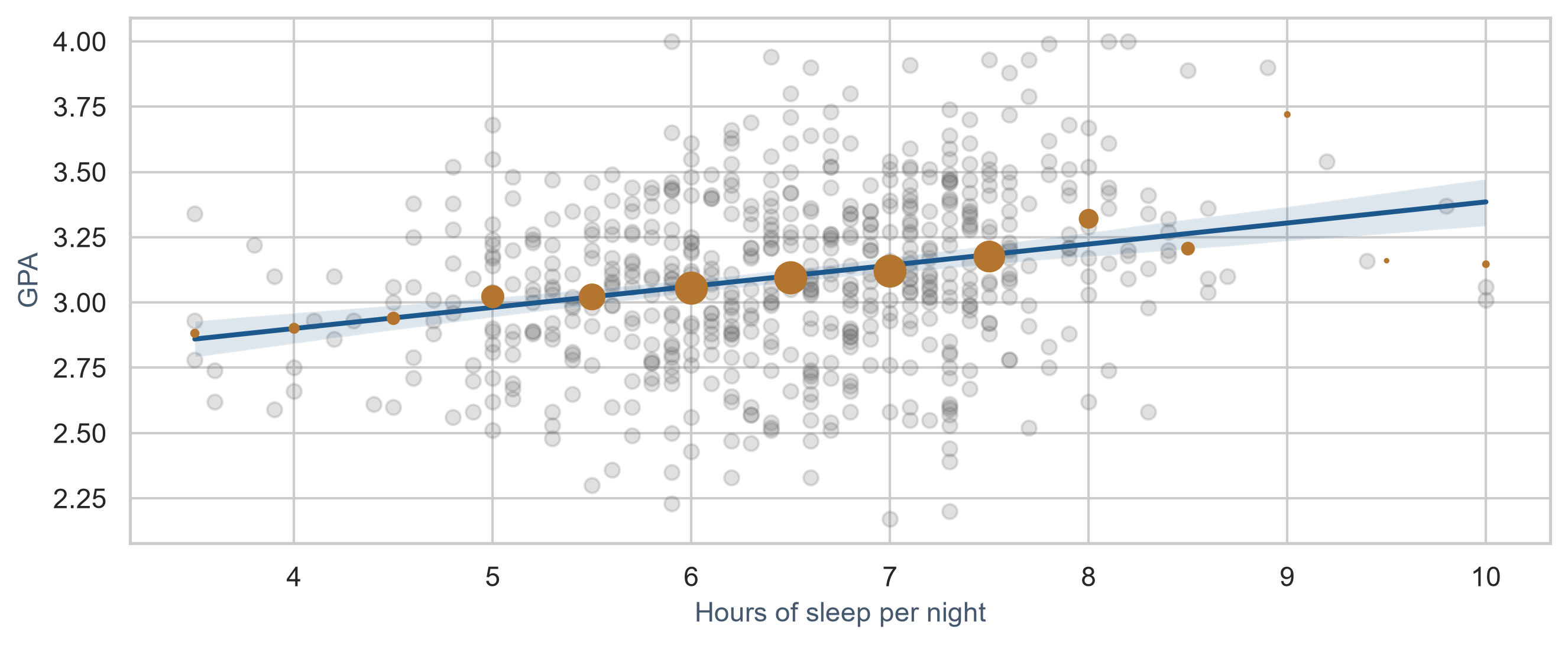
The spread of points around the line is what the model does not explain.
Simple linear regression
\[ \text{GPA} = b_0 + b_1 \times \text{sleep} + \text{error} \]
| Term | Meaning |
|---|---|
| \(b_0\), intercept | predicted GPA at zero sleep; places the line |
| \(b_1\), slope | change in predicted GPA per extra hour of sleep |
| residual | vertical distance from point to line |
Least squares minimizes the sum of squared residuals.
Fitting a line to five students
five = pd.DataFrame({"sleep": [5, 6, 6.5, 7, 8], "gpa": [2.8, 3.0, 3.2, 3.1, 3.4]})
fit_five = smf.ols("gpa ~ sleep", data=five).fit()
print(fit_five.params)
Each extra hour of sleep goes with a GPA about 0.18 points higher.
Nobody sleeps zero hours, so the intercept (1.91) rarely means anything on its own.
Three results in .summary()
| Result | Value | Meaning |
|---|---|---|
| slope | 0.08 | GPA gain per extra hour of sleep |
| R-squared (\(R^2\)) | 0.064 | share of GPA variation explained (~6%) |
| scale (RMSE) | 0.32 | typical distance from the line |
Sleep matters, but it is far from the whole story.
Multiple regression
gpa_model = smf.ols("gpa ~ sleep_hours + study_hours + stress + support", data=study).fit()
print(gpa_model.summary().tables[1])| Predictor | Slope (\(b\)) | Interpretation |
|---|---|---|
| sleep (hour) | +0.11 | holding study, stress, and support constant |
| study (hour a week) | +0.007 | holding others constant |
| stress (point) | -0.08 | holding others constant |
| support (point) | +0.11 | holding others constant |
Each coefficient holds the other predictors constant.
How much the model explains
\(R^2 = 0.252\) (25%): modest, and normal for human behavior and grades.
- Adjusted \(R^2\) (\(0.247\)) corrects for the number of predictors;
statsmodelsdrops rows with missing values (\(N = 587\) here).
Always report the number of cases each model is based on in your thesis.
Categorical predictors
gpa_gender = smf.ols(
    "gpa ~ sleep_hours + study_hours + stress + support + C(gender)",
    data=study
).fit()
print(gpa_gender.summary().tables[1])
Python compares each category with a reference category, alphabetically first: Female.
C(gender)[T.Male] is tiny (\(0.014\)) and non-significant (\(p = 0.56\)): no evidence that gender affects GPA.
To choose another reference: C(faculty, Treatment(reference='Humanities')).
Two explanations for caffeine and GPA
flowchart LR
  subgraph A["Caffeine as a cause"]
    C1[Caffeine] --> G1[GPA]
  end
  subgraph B["Sleep as a confounder"]
    S2[Sleep] --> C2[Caffeine]
    S2 --> G2[GPA]
    C2 -. "apparent link" .- G2
  end
Regression can tell them apart by comparing students who sleep the same amount.
Adjusting for the confounder
smf.ols("gpa ~ caffeine_mg", data=study).fit()
smf.ols("gpa ~ caffeine_mg + sleep_hours", data=study).fit()| Model | Caffeine slope | p-value |
|---|---|---|
| caffeine alone | -0.0004 | \(p < .001\) |
| with sleep added | -0.00008 | \(p = 0.51\) |
Among students who sleep the same, caffeine makes no difference to grades.
Regression adjusts only for what you include
A confounder is removed only if it was measured and put in the model.
Outside a randomised experiment, regression shows associations adjusted for the variables in the model, not proof of cause.
Curved relationships
gpa_curve = smf.ols("gpa ~ study_hours + np.power(study_hours, 2)", data=study).fit()
print(gpa_curve.summary().tables[1])
np.power(study_hours, 2) calculates the squared term before fitting.
The squared coefficient is negative and significant: the line bends downwards.
Diminishing returns
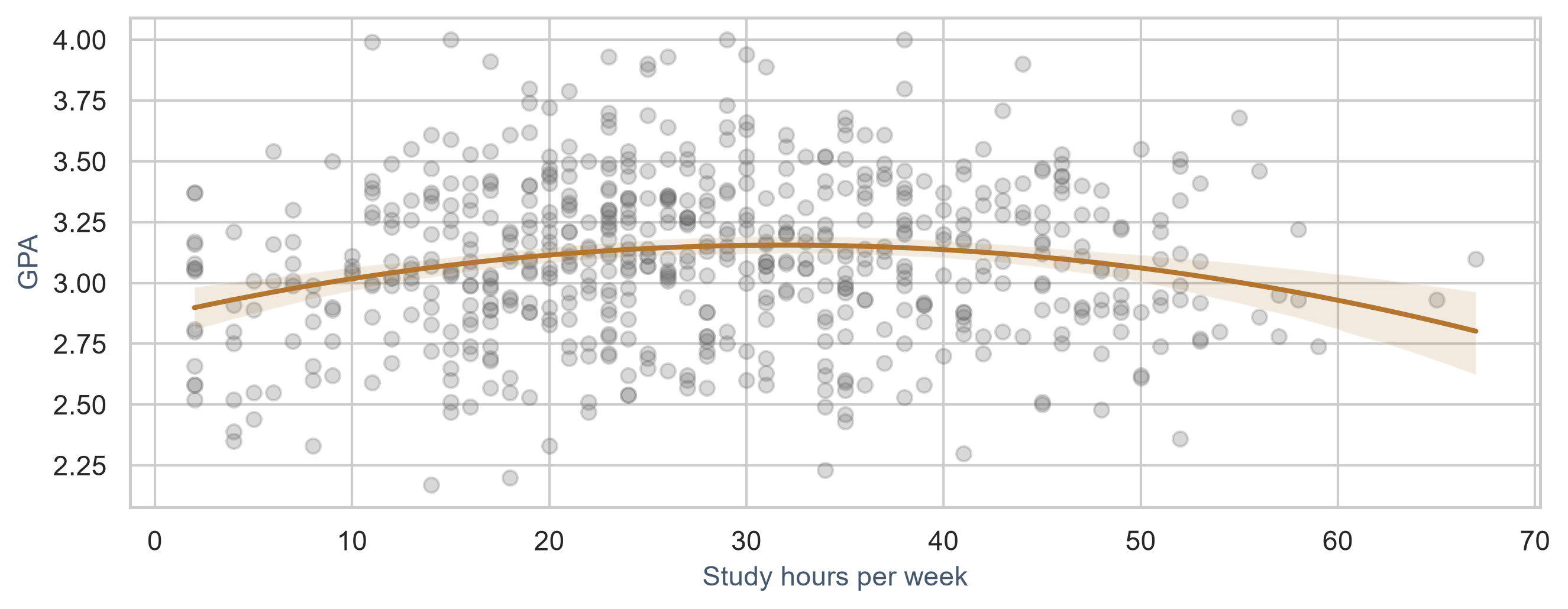
The first hours make a real difference. The curve peaks at about 32 hours a week.
Interactions in regression
study["support_c"] = study["support"] - study["support"].mean()
smf.ols("gpa ~ support_c * C(programme) + sleep_hours + study_hours", data=study).fit()Centring: zero now means average support.
| Programme | GPA change per point of support |
|---|---|
| Master’s | +0.07 |
| PhD | +0.13 |
Support matters about 1.8 times as much for PhD students.
What violated assumptions look like
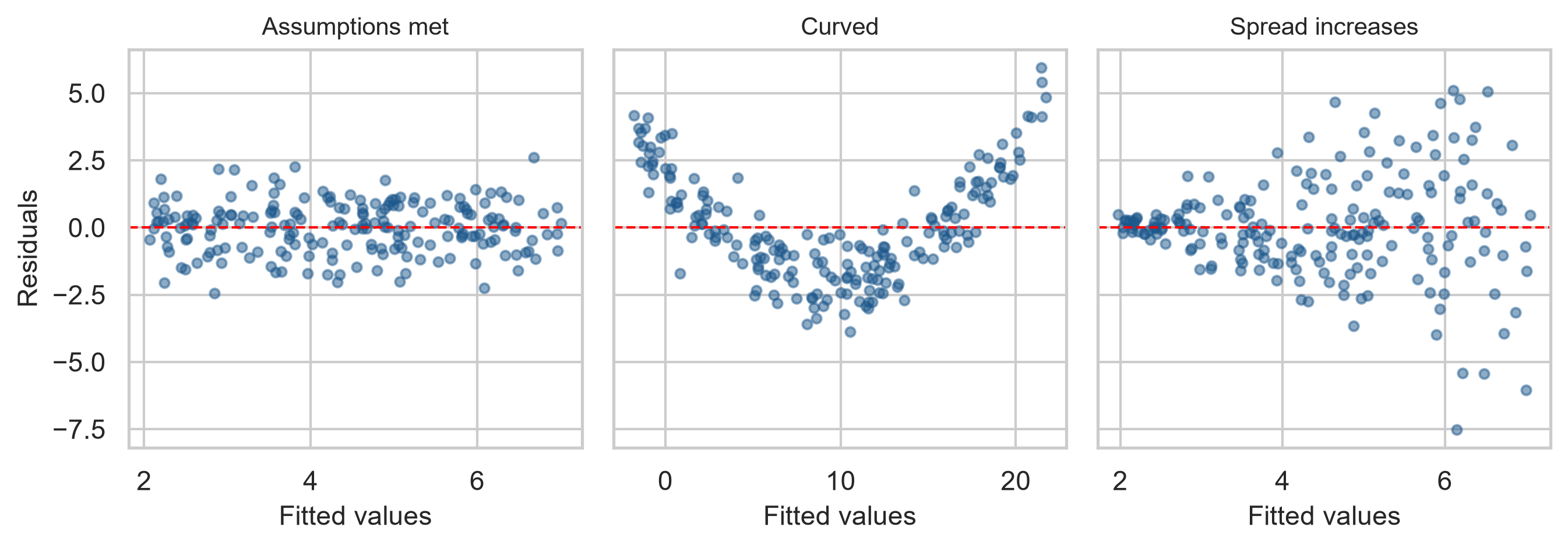
A shapeless band is good. A U shape means a missed curve. A funnel makes p-values unreliable.
Checking the GPA model
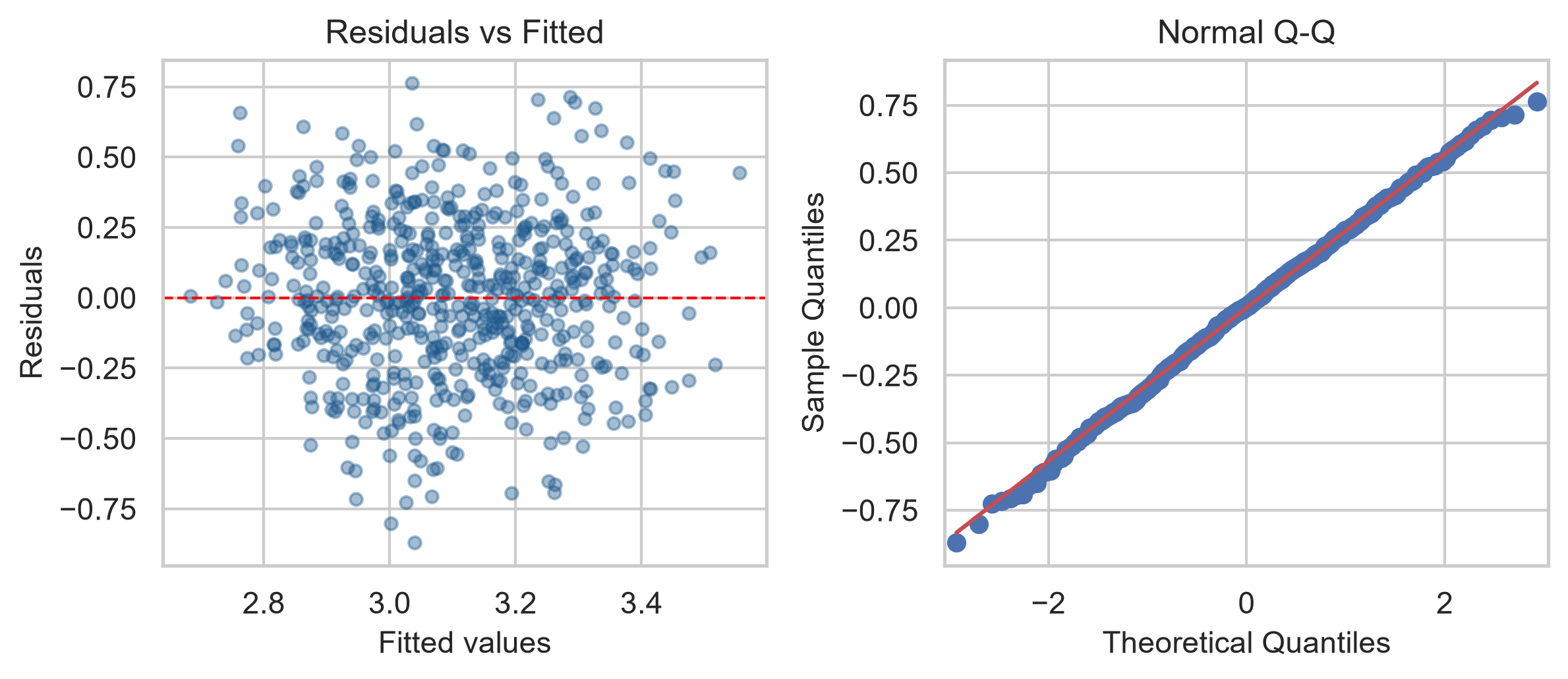
Residuals against fitted: a shapeless band, no curve, no funnel. Residual Q-Q: close to diagonal.
Writing it up in a thesis
A multiple regression of first-semester GPA on sleep, study hours, stress, and supervisor support explained 25% of the variance, F(4, 584) = 49.14, p < .001, N = 589. Holding the other predictors constant, each additional hour of sleep was associated with a GPA 0.15 points higher (95% CI [0.12, 0.18]).
The null hypothesis of a zero sleep coefficient was rejected.
Yes-or-no outcomes need logistic regression
Linear regression could predict probabilities below 0 or above 1.
Logistic regression models the probability of “yes” in a way that always stays between 0 and 1.
Odds and odds ratios
| Group | Odds of considering dropout |
|---|---|
| full-time job | 19 / 57 = 0.33 |
| no job | 41 / 266 = 0.15 |
| odds ratio | 0.33 / 0.15 = 2.2 |
1 means no difference; above 1 higher odds; below 1 lower odds.
A model for dropout
dropout_model = smf.logit(
    "dropout ~ stress + support + financial_worry + C(employment) + C(study_mode)",
    data=study
).fit()

odds_table = pd.DataFrame({
    "odds_ratio": np.exp(dropout_model.params),
    "ci_lower": np.exp(dropout_model.conf_int()[0]),
    "ci_upper": np.exp(dropout_model.conf_int()[1])
}).round(2)
print(odds_table)
The outcome is 0 or 1. np.exp() turns log-odds into odds ratios.
Reading the odds ratios
| Predictor (per point) | Odds ratio | 95% CI |
|---|---|---|
| stress | 3.60 | 2.25 to 5.77 |
| financial worry | 1.57 | 1.24 to 2.00 |
| support | 0.33 | 0.22 to 0.49 |
Stress multiplies odds by 3.6; support cuts them by about 67%. The stress hypothesis is strongly supported.
What happened to employment?
Alone, a full-time job about doubled the odds of considering dropout.
In the model, the employment intervals include 1 (comparing None vs Full-time, 95% CI [0.24, 1.31]).
A job likely matters because of the stress and money pressure it brings. Multiple regression makes that visible.
Predicted probabilities are easier to read
examples = pd.DataFrame({
    "stress": [2.5, 4.0], "support": [4.0, 2.0], "financial_worry": [3, 3],
    "employment": ["None", "None"], "study_mode": ["Full-time", "Full-time"]
})
dropout_model.predict(examples)| Student | Chance of considering dropout |
|---|---|
| low stress, good support | 4.0% |
| high stress, little support | 46.8% |
Explaining is not predicting
This model explains who considers dropping out.
Whether it can predict that for new students, and how to test that fairly, is a different question.
It is the subject of Chapters 11 and 12.
In your field: forestry and agriculture
tree_model = smf.ols("Volume ~ Girth + Height", data=trees).fit()
print(f"R-squared: {tree_model.rsquared:.2f}")
Timber volume of 31 black cherry trees from measurements taken without felling them.
Girth and height explain 95% of volume, against 25% for GPA: physics is more predictable than people.
Practical lab: the Chapter 8 playground
Work through the playground exercises in your browser, with hints and solutions.
Every exercise also runs in Python, from the downloadable chapter project.
Practical exercises 1–3: ANOVA and regression
- Wellbeing by faculty: ANOVA, \(\eta^2\), and Tukey if significant.
- Wellbeing on sleep: interpret the slope and R-squared.
- Add stress and support: what happens to the sleep slope and R-squared?
Practical exercises 4–6: categories, odds, confounders
- Add study mode: name the reference and interpret its coefficient.
- Dropout on burnout alone: report and explain the odds ratio.
- Draw a confounder from your own field, and say how regression would separate it.
Try this yourself
Choose one outcome in the student wellbeing data.
- plot it against one predictor;
- fit a simple regression, then add two plausible confounders;
- watch how the first coefficient changes;
- check the residual plot;
- write one sentence reporting the adjusted effect with its interval.
Troubleshooting guide (Part 1)
| Symptom | Likely cause |
|---|---|
| ten t-tests, one “significant” | multiple testing; use ANOVA and post-hoc tests |
| significant ANOVA, unclear which group | no post-hoc test |
| a coefficient changes sign when adding a predictor | a confounder, or correlated predictors |
| fewer cases than expected | statsmodels dropped rows with missing values |
Troubleshooting guide (Part 2)
| Symptom | Likely cause |
|---|---|
| a U shape in the residuals | a missed curve; add quadratic term |
| a funnel in the residuals | unequal spread; p-values unreliable; use robust SE |
| predicted probabilities above 1 | linear regression on a yes-or-no outcome |
| coefficients hard to explain to readers | log-odds not turned into odds ratios or probabilities |
Completion checklist
Misconceptions to leave behind (Part 1)
| Misconception | Better mental model |
|---|---|
| a significant coefficient shows a cause | an association adjusted for the model’s variables |
| a low R-squared makes a model useless | a real effect can explain little variation |
Misconceptions to leave behind (Part 2)
| Misconception | Better mental model |
|---|---|
| each coefficient describes its predictor alone | each holds the others constant |
| a significant ANOVA shows all groups differ | at least one differs; post-hoc tests say which |
The chapter in one sentence
ANOVA and regression split variation into what the predictors explain and what remains, and each coefficient holds the others constant, but only the ones you measured.
Next: Chapter 9
The next chapter looks at many variables at once:
- constructs and latent variables;
- principal component analysis (PCA);
- factor analysis of the questionnaire;
- reporting a questionnaire’s structure;
- cluster analysis for student profiles.
Questions
Which confounder could explain the main association in your own research?
Did you measure it?