flowchart TB
  subgraph R1[" "]
    direction LR
    A[Question] --> B[Import] --> C[Clean]
  end
  subgraph R2[" "]
    direction LR
    D[Explore] --> E[Test or predict] --> F[Report]
  end
  R1 --> R2
Descriptive Statistics and Exploratory Data Analysis
Descriptive Statistics and Exploratory Data Analysis
Say what you found, in the plainest sense
Chapter 6
Polla Fattah
By the end of today you can
- explain the place of exploratory analysis in research;
- choose a summary that suits the level and shape of a variable;
- summarise centre and spread, and explain standard deviation (including Pandas vs NumPy
ddof); - describe shape, and check it against the normal distribution;
- find unusual values, and decide what to do with them ethically;
- describe how much data is missing, and why (MCAR, MAR, MNAR);
- interpret correlations, and why correlation is not causation;
- describe a sample for a publication-ready thesis.
Description is not a formality
- the shape of a variable decides which tests are appropriate;
- an unusual value can dominate an analysis;
- missing data can quietly change who the results are about.
Descriptive statistics are the first results in almost every thesis.
Three kinds of analysis
| Kind | Purpose | Chapters |
|---|---|---|
| exploratory | gets to know the data; proves nothing | 6 |
| inferential | draws conclusions about a population | 7 to 10 |
| predictive | predicts new cases from existing patterns | 11 to 16 |
Exploration comes first
Return to exploration whenever a later inferential result surprises you.
Three measures of the centre
| Measure | Definition | Useful for |
|---|---|---|
| mean | the arithmetic average: sum divided by count | symmetrical numeric data |
| median | the middle value when sorted | skewed numeric data, ordinal data |
| mode | the most common value | categories (nominal data) |
\[ \bar{x} = \frac{1}{n} \sum_{i=1}^{n} x_i \]
One heavy user moves the mean
import pandas as pd

caffeine = pd.Series([0, 120, 150, 180, 900])
print("Mean:  ", caffeine.mean())    # 270.0
print("Median:", caffeine.median())  # 150.0
The mean (270 mg) is higher than four of the five students.
The mean is sensitive to extreme values; the median is robust.
Mean and median in the study
| Measure | Sleep (hours) | Caffeine (mg) |
|---|---|---|
| Mean | 6.5 | 152.8 |
| Median | 6.5 | 128.5 |
For sleep, mean and median match. For caffeine, the mean is pulled upward.
Why caffeine’s mean is higher
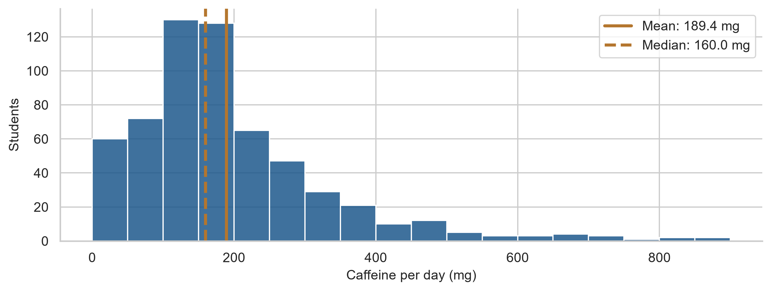
A minority of heavy users pulls the mean (solid) above the median (dashed).
Choosing a summary
| Variable | Centre | Spread | Examples |
|---|---|---|---|
| nominal | mode, percentages | none | faculty, gender |
| ordinal | median, percentages | IQR | financial worry, Likert items |
| numeric, symmetrical | mean | SD | sleep, wellbeing |
| numeric, skewed | median | IQR | caffeine, age |
The level of measurement comes first, then the shape.
Same average, different stories
group_a = pd.Series([6.0, 6.5, 6.5, 7.0, 6.5])
group_b = pd.Series([4.0, 8.5, 5.0, 9.0, 6.0])

print(group_a.mean(), group_b.mean())  # Both 6.5 hours
Both average 6.5 hours.
In group A everyone sleeps about the same; group B ranges from 4 to 9 hours.
A mean without a measure of spread hides half the story.
Deviations from the mean
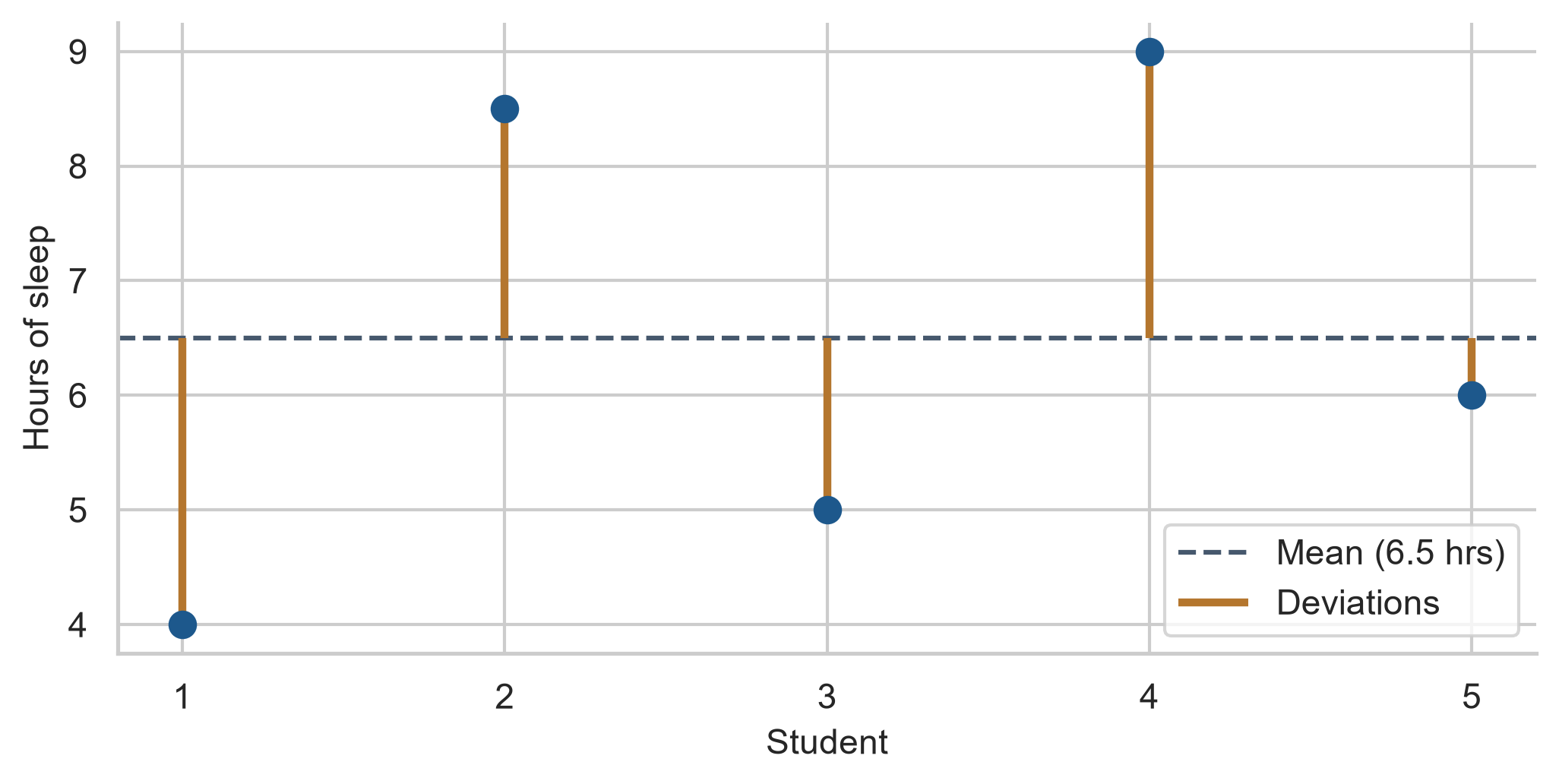
Each copper line is a deviation, \(x_i - \bar{x}\). The standard deviation summarises them.
The standard deviation
\[ s = \sqrt{\frac{1}{n-1} \sum_{i=1}^{n} (x_i - \bar{x})^2} \]
- deviations add to zero, so they are squared first;
- the average squared deviation is the variance;
- its square root returns to the original units.
Dividing by \(n - 1\) (Bessel’s correction) gives an unbiased estimate from sample data.
Crucial Python Detail: ddof
- Pandas
s.std()usesddof=1(\(n-1\)) by default (sample statistic). - NumPy
np.std(x)usesddof=0(\(n\)) by default (population statistic).
print("Pandas: ", group_b.std())          # 2.12
print("NumPy:  ", np.std(group_b))        # 1.90
print("Correct:", np.std(group_b, ddof=1)) # 2.12
Always use ddof=1 for sample standard deviations in research.
The SD is roughly the typical distance
print(group_a.std())                       # 0.35 hours
print(group_b.std())                       # 2.12 hours
print((group_b - group_b.mean()).abs().mean())  # 1.80 hours (mean deviation)
Group B’s SD is close to the average length of the copper lines.
It is a little larger because squaring weights the longest lines more heavily.
The interquartile range
q1 = first_sem["caffeine_mg"].quantile(0.25)  # 105 mg
q3 = first_sem["caffeine_mg"].quantile(0.75)  # 240 mg
iqr = q3 - q1                                  # 135 mg
The spread of the middle half: \(Q_3 - Q_1\). It ignores the extremes, like the median.
A box plot’s box is exactly the IQR.
Pairs that belong together
| Centre | Spread |
|---|---|
| mean | standard deviation (SD) |
| median | interquartile range (IQR) |
Sleep: SD ≈ 1.0 hours, so a typical student sleeps within about an hour of 6.5 hours.
The shape of a distribution
| Shape | Meaning | Mean and median |
|---|---|---|
| symmetrical | two sides mirror each other | about equal |
| skewed right | a long tail of high values | mean above median |
| skewed left | a long tail of low values | mean below median |
| bimodal | two peaks | often two groups mixed |
Sleep is symmetrical, caffeine is not
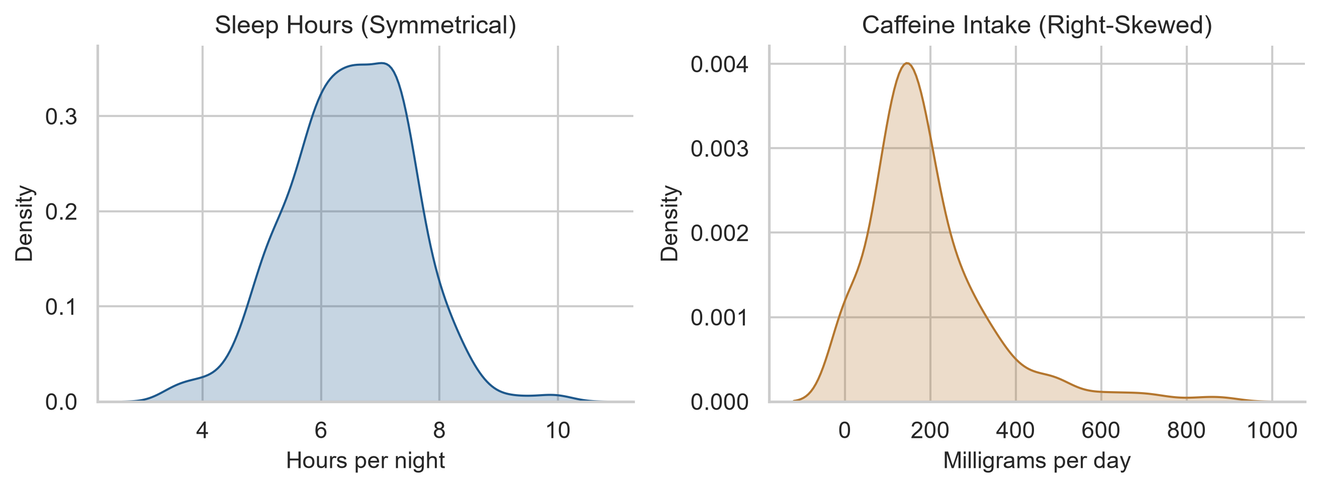
Skewness puts a number on it
print("Sleep:   ", first_sem["sleep_hours"].skew().round(2))  # -0.05
print("Caffeine:", first_sem["caffeine_mg"].skew().round(2))  #  1.27
print("Age:     ", students["age"].skew().round(2))           #  1.18
0 is symmetrical, positive a tail to the right. Between −1 and +1 is mild.
Most graduate students are in their twenties; fewer are older.
The normal distribution
Symmetrical and bell-shaped, described completely by its mean and SD.
Many tests assume data, or averages of data, follow it approximately (Chapter 7).
| Within | Share of values |
|---|---|
| 1 SD of the mean | about 68% |
| 2 SD | about 95% |
| 3 SD | about 99.7% |
Checking sleep against the rule
z = (first_sem["sleep_hours"] - sleep_mean) / sleep_sd

print((z.abs() < 1).mean().round(3))  # 0.678 (≈ 68%)
print((z.abs() < 2).mean().round(3))  # 0.957 (≈ 95%)
print((z.abs() < 3).mean().round(3))  # 0.998 (≈ 99.7%)
Very close to 68-95-99.7.
z-scores give each value’s distance from the mean in standard deviations:
\[ z_i = \frac{x_i - \bar{x}}{s} \]
Q-Q plots compare with the normal
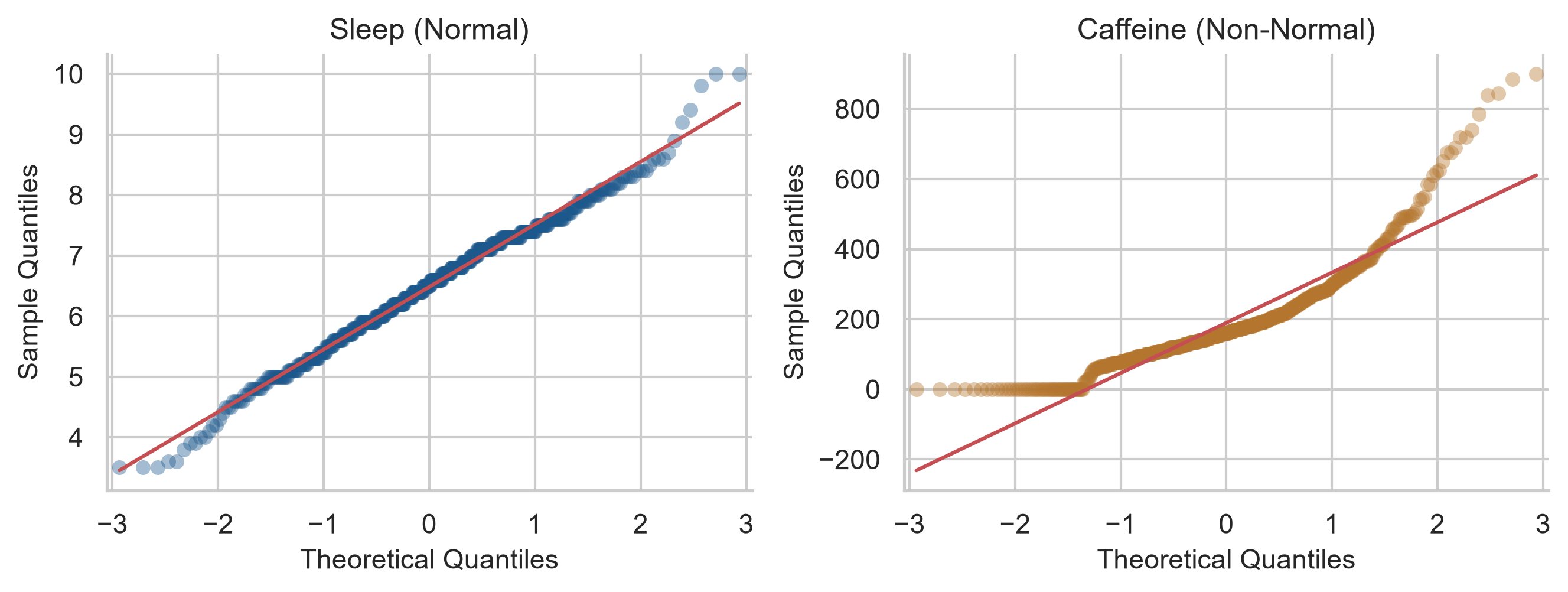
Sleep sits on the line. Caffeine bends away at the top: its long right tail.
Outliers are information first
Impossible values were set to np.nan in Chapter 3. Outliers are possible, just unusual.
An unusual value may be: - an error that cleaning missed; - a participant who misunderstood a question; - a real case the research should pay attention to.
Find them and look at them before anything else.
Two rules for flagging
| Rule | Flags values | Suits |
|---|---|---|
| box plot rule (Tukey) | beyond 1.5 × IQR from the quartiles | skewed variables |
| z-score rule | more than 3 SD from the mean (\(|z| > 3\)) | roughly normal variables |
The box plot rule for caffeine
q1 = first_sem["caffeine_mg"].quantile(0.25)
q3 = first_sem["caffeine_mg"].quantile(0.75)
upper_fence = q3 + 1.5 * (q3 - q1)

print("Upper fence:", upper_fence)                         # 442.5 mg
print("Outliers:   ", (first_sem["caffeine_mg"] > upper_fence).sum()) # 35
35 students consume more than the upper fence of 442.5 mg.
For sleep (normal), the z-score rule flags 2 students.
The most extreme cases
first_sem.query("sleep_hours <= 4.5 and caffeine_mg >= 600")[
    ["student_id", "sleep_hours", "caffeine_mg", "study_hours", "wellbeing"]
]
These students sleep 3.5 to 4.3 hours, take 610 to 900 mg of caffeine, and study up to 67 hours a week.
Nothing impossible: a real and worrying group, exactly what the thesis is about.
Never delete a value just because it is unusual
- Check whether it is an error (Chapter 3).
- If it is real, keep it and report it.
- Choose summaries that are not distorted by it, such as the median.
- Check whether conclusions change without it: a sensitivity analysis.
Removing inconvenient values for a cleaner result is research misconduct.
Count the gaps first
About 1% of each semester measurement is missing.
38 students did not answer the question about financial worries.
Why data is missing matters more than how much
| Kind | The gaps depend on | Consequence |
|---|---|---|
| missing completely at random (MCAR) | nothing | unbiased, a little less precise |
| missing at random (MAR) | something measured | correctable by including it |
| missing not at random (MNAR) | the missing value itself | the respondents left are not typical |
Students most worried about money may be the least willing to say so.
The biggest gap: students who left
sem3_students = set(semesters.query("semester == 3")["student_id"])
left_ids = set(students["student_id"]) - sem3_students

first_sem["left_study"] = first_sem["student_id"].isin(left_ids)
first_sem.groupby("left_study").agg(
    students=("student_id", "count"),
    wellbeing=("wellbeing", "mean"),
    considering_dropout=("considering_dropout", lambda s: (s == "Yes").mean() * 100)
).round(1)| Group | Students | Wellbeing | Considered dropout |
|---|---|---|---|
| Stayed | 548 | 53.6 | 14.1% |
| Left | 52 | 45.3 | 63.5% |
What attrition does to later semesters
The students still present in semesters 3 and 4 were, on average, doing better.
A simple average of the later semesters overestimates how well students were doing: survivorship bias.
- report how many left and how they differed;
- mixed models (Chapter 10) use every observation each student gave;
- multiple imputation exists for large missingness gaps.
The correlation coefficient
\(r\) measures how closely two numeric variables follow a straight line, from −1 to +1.
| \(r\) (either sign) | Conventional benchmark (Cohen 1988) |
|---|---|
| about 0.10 | small |
| about 0.30 | medium |
| about 0.50 | large |
Rough guides, not rigid rules. A curved relationship can have \(r\) near zero.
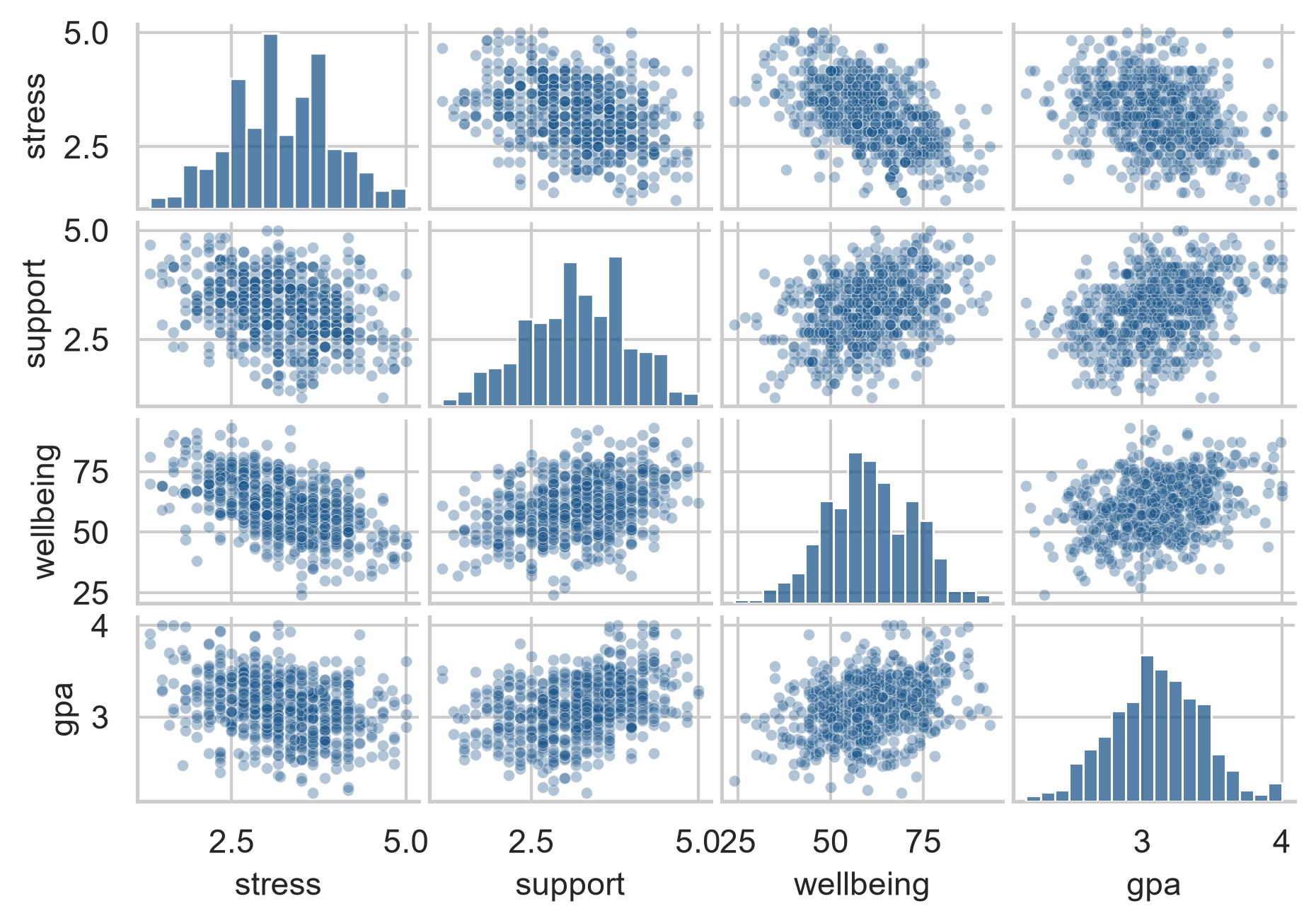
A correlation matrix
| Construct | Burnout | Support | Wellbeing | GPA |
|---|---|---|---|---|
| Stress | 0.62 | −0.34 | −0.51 | −0.29 |
| Support | −0.22 | 1.00 | 0.34 | 0.28 |
Stress and burnout correlate strongly; supervisor support associates with lower stress and higher GPA.
A scatter plot matrix
Correlation is not causation
flowchart LR
    S["Less sleep"] --> C["More caffeine"]
    S --> G["Lower GPA"]
    C -. "correlation −0.21" .- G
Caffeine may only look harmful because heavy caffeine consumers sleep less: a confounder (Chapter 8).
Describing the sample
pd.Series({
    "N": len(first_sem),
    "Female (%)": (first_sem["gender"] == "Female").mean() * 100,
    "PhD (%)": (first_sem["programme"] == "PhD").mean() * 100,
    "Part-time (%)": (first_sem["study_mode"] == "Part-time").mean() * 100,
    "Age Mean": first_sem["age"].mean(),
    "Age SD": first_sem["age"].std()
}).round(1)
Who took part: the first table in the methodology chapter.
Every summary needs its spread and its n
A mean of 6.4 hours says little until the reader knows: - whether students differ by minutes or by hours; - whether it comes from 20 students or 600.
With missing values, valid \(n\) differs from variable to variable, so report it for each.
Description table for main variables
def describe_var(s):
    v = s.dropna()
    return pd.Series({
        "n": len(v), "mean": v.mean(), "sd": v.std(),
        "median": v.median(), "iqr": v.quantile(0.75) - v.quantile(0.25),
        "missing": s.isna().sum()
    })

first_sem[["sleep_hours", "study_hours", "caffeine_mg", "gpa", "wellbeing"]].apply(describe_var).T.round(2)
Writing it up
The sample consisted of 600 graduate students (50% female; 50% PhD candidates), aged 22 to 52 years (M = 29.7, SD = 4.8). Students reported sleeping an average of 6.5 hours per night (SD = 1.1), with 68% sleeping fewer than 7 hours.
Every number comes directly from Python code.
An exploration checklist
- How many values are missing, and why?
- What is the typical value, and how spread out are the observations?
- What is the shape: symmetrical or skewed, unimodal or multimodal?
- Are there unusual values, and are they errors or genuine?
- How does the variable relate to other measures?
In your field: earth sciences
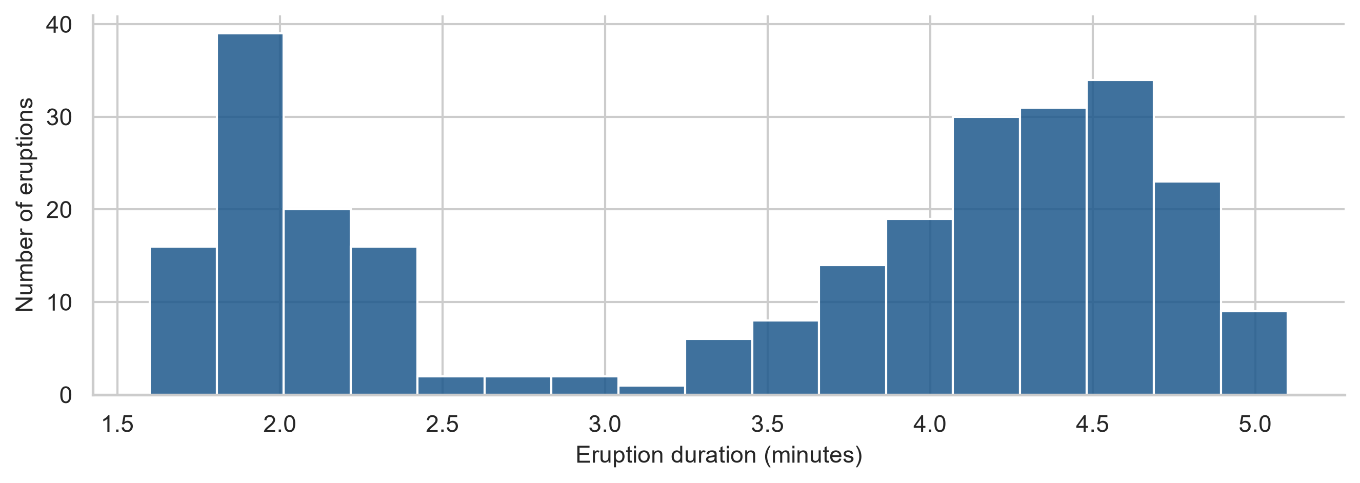
Old Faithful: eruptions last about 2 or about 4.5 minutes. The mean (3.5 min) describes almost none of them. Report the two regimes separately.
Practical lab: Chapter 6 playground
Work through the playground exercises in your browser with interactive Pyodide feedback.
Every exercise also runs locally in VS Code with the downloadable project zip (chapter06.zip).
Misconceptions to leave behind
| Misconception | Better mental model |
|---|---|
| the mean is the typical value | only for roughly symmetrical variables |
| a mean on its own is a result | it needs its spread and valid n |
| outliers should be removed | real values are reported and handled |
| a few missing values do not matter | why they are missing matters far more |
| \(r = 0\) means no relationship | no straight-line relationship |
| correlation shows causation | a confounder can create it |
The chapter in one sentence
Describe every variable by its centre, spread, shape, gaps, and unusual values before you test anything.
Next: Chapter 7
The next chapter moves from descriptive exploration to statistical inference: - sampling distributions and standard errors; - confidence intervals and the bootstrap; - the logic of a hypothesis test, built by shuffling; - independent \(t\)-tests, effect sizes, and chi-square tests in Python.