flowchart TD
  A["Topic: graduate student wellbeing"] --> B["Problem: many report stress; some leave"]
  B --> C["Focus: can the university do something?"]
  C --> D["Question: does a six-week workshop improve<br>wellbeing by the end of the next semester?"]
From Research Question to Data
From Research Question to Data
Deciding what you are asking before any statistics
Chapter 5
Polla Fattah
By the end of today you can
- explain what data analysis is for: describing, explaining, predicting;
- turn a broad topic into a focused research question;
- write a falsifiable hypothesis and its corresponding null hypothesis;
- turn an abstract construct into a measured variable and judge its measurement level;
- identify the distinct roles variables play in an analytical model;
- distinguish measurement reliability from construct and study validity;
- determine what each study design can and cannot establish;
- explain why a biased sample cannot be fixed by making it larger;
- plan an analysis and calculate necessary sample size (statistical power) before data collection.
Most thesis problems start before the analysis
- a question too vague to answer empirically;
- a hypothesis no data could possibly contradict;
- a questionnaire that measures something other than what the thesis promises;
- a convenience sample that cannot support generalizable conclusions.
No statistical test or machine learning algorithm can fix these afterwards.
Data analysis tests claims against evidence
| Aim | Example question | Judged by |
|---|---|---|
| Describe | How long do graduate students sleep? | Accuracy, and who the summary applies to |
| Explain | Does the workshop improve wellbeing? | Whether rival explanations are ruled out |
| Predict | Who will consider dropping out? | Accuracy on new unseen cases |
Describing: Chapters 4, 6, 7. Explaining: Chapters 7 to 10. Predicting: Chapters 11 to 16.
The same model, different aims
A multiple regression model can explain GPA: which predictors matter, and how much?
The exact same model can predict GPA: how close are predictions for incoming students?
The mathematical specification may be identical. The research goal, and how success is evaluated, are fundamentally different.
From a topic to a research question
A research question is a broad topic narrowed until empirical data can answer it.
A good research question is
- specific: names who, what, and when;
- answerable with data you can feasibly collect;
- not already answered in the existing literature;
- feasible within your time, budget, skills, and ethical access;
- worth answering: someone would make a different practical decision depending on the outcome.
Weak questions, improved
| Weak question | Underlying problem | Better question |
|---|---|---|
| Are students stressed? | Compared with what? | Do part-time students report higher stress than full-time students? |
| What affects success? | “Success” is undefined | Is semester sleep associated with GPA, allowing for study hours? |
| Is the workshop good? | “Good” is unmeasurable | Does the workshop raise wellbeing by the end of semester 2? |
| Why do students drop out? | Requires years of tracking | Which baseline traits are associated with considering dropout? |
Three kinds of question
| Kind | Asks | Data needed | What it can claim |
|---|---|---|---|
| Descriptive | What is? | Representative sample | Population summary |
| Relational | What goes with what? | Both variables measured | Statistical association |
| Causal | What leads to what? | Design ruling out alternatives | Cause and effect |
Asking a relational question and answering in causal words (“sleep improves grades”) is one of the most common errors in empirical theses.
A hypothesis answers in advance
Hypothesis: Students invited to the workshop will report higher wellbeing at the end of semester 2 than students not invited.
A research question asks. A hypothesis states the best a priori prediction grounded in theory and earlier literature.
It is scientifically valuable precisely because the empirical data can disagree with it.
Falsifiability (Popper)
| Hypothesis | Could any empirical result contradict it? |
|---|---|
| “The workshop affects students in some way.” | No: higher, lower, or identical wellbeing all fit. Unfalsifiable. |
| “It helps students who are ready for it.” | No, unless “ready” is objectively defined in advance. |
| “Invited students will have higher wellbeing.” | Yes: equal or lower wellbeing contradicts it. Falsifiable. |
Karl Popper (1959): What makes an assertion scientific is that it forbids certain outcomes.
Write down what would count against you
Before viewing any data, explicitly name the finding that would contradict your hypothesis.
If you cannot name what would prove you wrong, your question is not yet precise enough for scientific research.
If you pre-commit to refutation criteria, you are protected against rationalizing disappointing results after the fact.
Four properties of a good hypothesis
- Formulated about a stated population and operationalized variables;
- Testable with accessible, ethical data;
- Falsifiable: pre-specifies the empirical result that would contradict it;
- Stated before the data is collected and analysed.
A hypothesis conceived after inspecting data merely summarizes that specific sample—it does not test a theory.
Directional vs non-directional hypotheses
| Kind | What it predicts | Example |
|---|---|---|
| Directional | Specific sign/direction of effect | Invited students will report higher wellbeing |
| Non-directional | Difference exists, direction unstated | Stress scores will differ across faculties |
Directional hypotheses make stronger scientific claims because they forbid more potential outcomes.
The null hypothesis (\(H_0\))
| Hypothesis | Operational statement for the workshop |
|---|---|
| \(H_1\) (Alternative) | Invited and uninvited students differ in average wellbeing |
| \(H_0\) (Null) | The two groups have the same population mean wellbeing (\(\mu_1 = \mu_2\)) |
\(H_0\) provides a mathematically exact baseline: any observed group difference is attributable to random sampling variation alone.
Simulating the null world
np.random.seed(2026)
chance_diffs = []
groups = np.repeat(["Invited", "Not invited"], 150)

for _ in range(5000):
    wb = np.random.normal(loc=60, scale=11, size=300)
    shuffled = np.random.permutation(groups)
    diff = wb[shuffled == "Invited"].mean() - wb[shuffled == "Not invited"].mean()
    chance_diffs.append(diff)
300 imaginary students, a workshop that does nothing, two random groups, repeated 5,000 times.
Chance alone produces differences
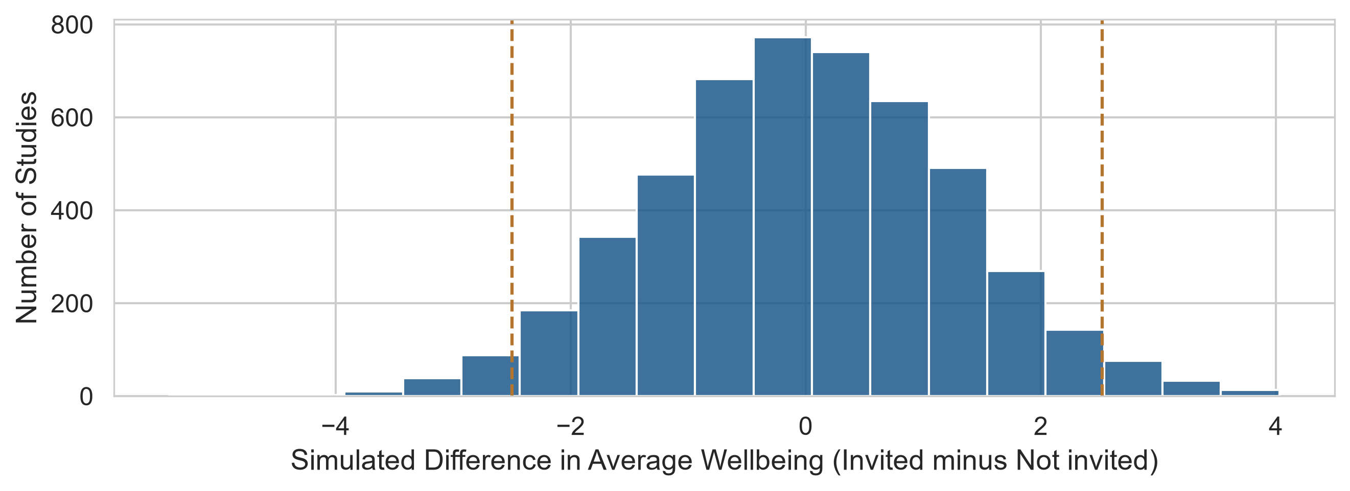
95% of chance differences fall between -2.5 and 2.5. An observed 5-point difference is highly unlikely under chance alone (\(p < .05\)); a 1-point difference is completely routine.
What a hypothesis test can and cannot conclude
- Rejecting \(H_0\) is NOT proving \(H_1\): it demonstrates only that “pure chance” is an implausible explanation of the data.
- Failing to reject \(H_0\) is NOT proving \(H_0\): an underpowered study can easily fail to detect a real effect.
A blurry photograph can fail to reveal a face, but that does not prove the person was absent.
Confirmatory vs exploratory research
| Mode | What it does | Result status |
|---|---|---|
| Confirmatory | Tests an a priori hypothesis specified in advance | Confirms or refutes a prediction |
| Exploratory | Uncovers patterns with no prior expectation | Generates new hypotheses for future studies |
Both modes are scientifically vital, provided they are reported transparently and not conflated.
Think before you analyse
Before executing any analytical code, answer these four questions in writing:
- What is the research question: descriptive, relational, or causal?
- What is the unit of analysis: individual students, repeated semesters, or supervisors?
- Which variables, at what measurement levels, serve as outcomes and predictors?
- What exact empirical finding would support the hypothesis, and what would refute it?
The unit of analysis decides what a row means
len(students)      # 600: one row per student
len(semesters)     # 2,326: one row per student per semester
len(supervisors)   # 120: one row per faculty supervisor
“Do students who sleep more have higher GPAs?” is a question about individual students.
Treating 2,326 longitudinal semester rows as independent observations would artificially inflate statistical significance (Chapter 10).
Constructs require operationalisation
Stress, wellbeing, intellectual engagement: latent constructs that cannot be physically inspected.
Operationalisation specifies the measurement procedure that translates a construct into concrete data.
Every operationalisation involves trade-offs; an alternative instrument could yield different findings.
Operationalising the wellbeing study
| Construct | Operational measurement | Dataset variable |
|---|---|---|
| Sleep | Self-reported mean hours per night in semester | sleep_hours |
| Stress | Mean score of six 1-to-5 Likert survey items | stress_1 to stress_6 |
| Wellbeing | Validated 0-to-100 multidimensional index | wellbeing |
| Performance | Cumulative Grade Point Average from records | gpa |
| Dropout thoughts | “Have you seriously considered leaving?” | considering_dropout |
Operationalising the stress scale
stress_items = [f"stress_{i}" for i in range(1, 7)]
q_stress = questionnaire[stress_items].copy()
q_stress["stress_4"] = 6 - q_stress["stress_4"]  # reverse code item 4

stress_score = q_stress.mean(axis=1)
No single questionnaire item adequately captures stress, so six indicators are averaged.
Item 4 is reverse-worded and must be inverted before aggregation.
Levels of measurement (Stevens, 1946)
| Level | Properties | Permissible statistics | Pandas dtype |
|---|---|---|---|
| Nominal | Unordered categories | Counts, proportions, mode | object, category |
| Ordinal | Ranked order; unknown intervals | Median, percentiles | category(ordered=True) |
| Interval | Equal intervals; arbitrary zero | Mean, SD, linear diffs | float64 |
| Ratio | Equal intervals; true physical zero | Ratios, geometric mean | float64, int64 |
Averaging nominal categories is meaningless. Ratio claims (“twice as high”) are invalid on interval indices.
Declaring categorical order in Pandas
students["employment"] = pd.Categorical(
    students["employment"],
    categories=["None", "Part-time job", "Full-time job"],
    ordered=True
)
By default, Python sorts text alphabetically, placing “Full-time job” before “None”.
Declaring an ordered pd.Categorical ensures tables, plots, and logical filters (> "None") respect the natural hierarchy.
The roles variables play
| Role | Meaning in model | Case study example |
|---|---|---|
| Outcome | What is explained or predicted (\(Y\)) | Wellbeing, GPA |
| Predictor | What explains or predicts (\(X\)) | Workshop condition, sleep |
| Confounder | Causes both \(X\) and \(Y\); creates spurious link | Sleep duration (for caffeine and GPA) |
| Moderator | Alters the strength/direction of \(X \to Y\) | Academic programme (Master’s vs PhD) |
| Mediator | Intermediate mechanism on causal pathway | Reduced stress linking workshop to wellbeing |
Three roles of a third variable
flowchart LR
  subgraph Confounder
    S1[Sleep] --> C1[Caffeine]
    S1 --> G1[GPA]
    C1 -. "spurious link" .- G1
  end
  subgraph Mediator
    W[Workshop] --> ST[Lower stress] --> WB[Wellbeing]
  end
A moderator (e.g., degree programme) alters the magnitude of an existing relationship without being caused by the predictor.
Confounding in the empirical data
caffeine_mg |
sleep_hours |
gpa |
|
|---|---|---|---|
caffeine_mg |
1.00 | −0.64 | −0.18 |
sleep_hours |
−0.64 | 1.00 | 0.25 |
Caffeine correlates negatively with GPA, but also correlates heavily with sleep loss.
Chapter 8 uses multiple regression to compare caffeine effects among students with identical sleep.
Reliability vs validity
| Attribute | Core question | Stress scale example |
|---|---|---|
| Reliability | Is the measurement consistent? | Similar score on re-test; internal items correlate |
| Validity | Does it measure the intended construct? | Captures psychological stress, not momentary tiredness |
Target analogy
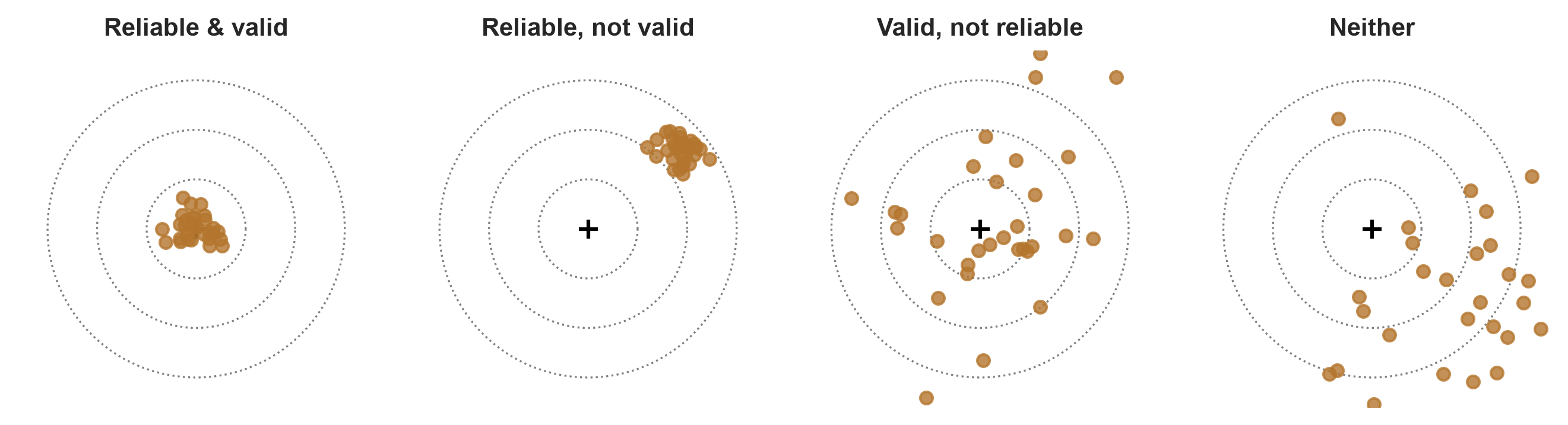
Reliability is necessary for validity, but not sufficient: a scale always two kilograms too heavy is consistent but systematically wrong.
Checking construct validity
| Stress | Burnout | Support | Satisfaction | |
|---|---|---|---|---|
| Stress | 1.00 | 0.65 | −0.33 | −0.41 |
Stress exhibits convergent validity with burnout (\(r = 0.65\)) without being redundant, and discriminant validity with satisfaction (\(r = -0.41\)).
Reporting construct correlations in thesis methodology establishes measurement credibility.
Study designs and causal inference
| Design | Can it show causality? | Role in the wellbeing study |
|---|---|---|
| Randomised experiment | Yes, for the manipulated treatment | The workshop invitation |
| Quasi-experiment | Only with extensive control | Students who chose session attendance |
| Cross-sectional | No; correlation only | Baseline questionnaire |
| Longitudinal | Establishes temporal sequence | The four repeated semester waves |
Research design, not statistical technique, governs causal claims.
Self-selection bias
If the workshop had been open to voluntary sign-ups, motivated students with lower baseline stress would have volunteered.
Any later wellbeing advantage would conflate the intervention’s benefit with pre-existing personal attributes.
Simulating self-selection vs randomisation
chance_to_volunteer = expit(-2 * (stress_scores - stress_scores.mean()))
volunteered = np.random.uniform(size=600) < chance_to_volunteer
invited = np.random.permutation(np.repeat([True, False], 300))| Design strategy | Baseline stress difference between groups |
|---|---|
| Voluntary self-selection | −0.80 points (volunteers enter less stressed) |
| Random invitation | +0.06 points (groups enter effectively identical) |
Random assignment balances the unmeasured
| Group | \(n\) | Mean Age | % Female | % PhD | Financial Worry | Baseline Stress |
|---|---|---|---|---|---|---|
| Invited | 300 | 29.6 | 50.3% | 28.7% | 2.8 | 3.2 |
| Not invited | 300 | 29.8 | 53.7% | 29.3% | 2.9 | 3.2 |
Randomization balances measured traits AND unmeasured confounders (grit, family support, coping skills).
A baseline equivalence table is required in any experimental thesis.
Random error vs sampling bias
| Property | Source | Response to larger sample |
|---|---|---|
| Random error | Chance variation in who was selected | Decreases with larger sample (\(SE \propto 1/\sqrt{n}\)) |
| Sampling bias | Flawed recruitment or self-selection | Does not decrease; wrong answer with more certainty |
A biased sample cannot be fixed by size
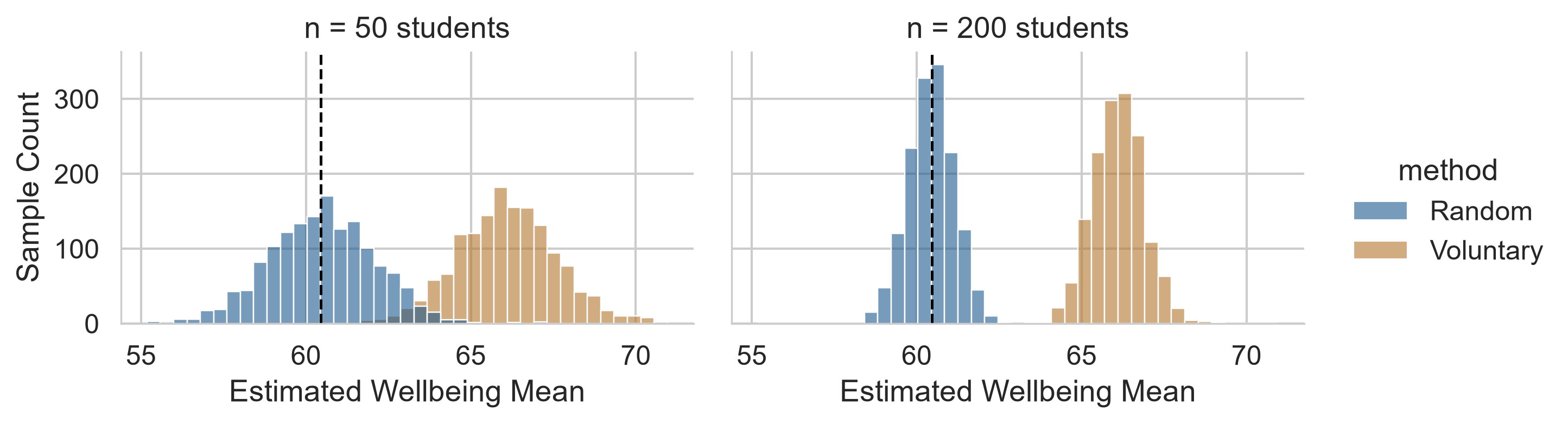
Larger sample sizes narrow the distribution width; they do not shift a biased estimate toward the true population parameter.
Statistical power and sample size planning
Statistical power depends on:
- Sample size (\(N\));
- True population effect size (e.g., Cohen’s \(d\));
- Significance threshold (\(\alpha\)).
Power (\(1 - \beta\)) is the probability of detecting an effect of a given magnitude if it genuinely exists (standard benchmark: 80%).
Calculating sample size in Python
from statsmodels.stats.power import TTestIndPower

power_analyzer = TTestIndPower()
required_n = power_analyzer.solve_power(
    effect_size=0.45,
    power=0.80,
    alpha=0.05,
    alternative="two-sided"
)
Detecting a moderate effect (\(d = 0.45\)) requires approximately 79 participants per group (\(N = 158\)).
Smaller effects require drastically larger samples
effect_sizes = {"small (0.2)": 0.2, "medium (0.5)": 0.5, "large (0.8)": 0.8}
{name: int(np.ceil(power_analyzer.solve_power(d, power=0.80, alpha=0.05)))
for name, d in effect_sizes.items()}| Effect size | Cohen’s \(d\) | Required \(n\) per group |
|---|---|---|
| Small | 0.20 | 393 students |
| Medium | 0.50 | 64 students |
| Large | 0.80 | 26 students |
Halving the target effect size roughly quadruples the necessary sample size.
Preregistration
Analytical choices (exclusions, covariate controls, outlier winsorization) made post-hoc can unconsciously bias results toward statistical significance.
Preregistration creates an unalterable, time-stamped record of hypotheses and analysis plans before observing outcome data.
It does not prohibit exploratory discovery; it simply ensures that exploratory findings are acknowledged as such.
Practical lab: Chapter 5 playground
Practice the concepts in the browser playground or your local VS Code environment:
- A. Practise the chapter: Formulate falsifiable hypotheses, define ordered categoricals, simulate small-sample null worlds, verify baseline equivalence, and run power calculations.
- B. Go further: Evaluate stratified sampling stability, simulate correlation power, and examine biased estimators.
- C. Check your understanding: Core conceptual definitions.
- D. Do it yourself: Design an analysis plan and pilot power evaluation.
The chapter in one sentence
Formulate a specific, falsifiable question, establish your operational measures, and justify your research design and sample size before inspecting the empirical data.
Next: Chapter 6
Moving from study design to empirical exploration:
- Central tendency, dispersion, and distribution skewness;
- Identifying and managing extreme outliers responsibly;
- Diagnosing missing data patterns and longitudinal attrition;
- Generating professional sample description tables for publication.
Questions & Discussion
What empirical result would count as definitive evidence against your thesis hypothesis?
Does your intended sample size provide sufficient statistical power to detect that outcome?